Thongchai Thailand

“The Kuwaiti oil fires were caused by Iraqi military forces setting fire to a reported 605 to 732 oil wells along with an unspecified number of oil filled low-lying areas, such as oil lakes and fire trenches, as part of a scorched earth policy while retreating from Kuwait in 1991 due to the advances of Coalition military forces in the Persian Gulf War. The fires were started in January and February 1991, and the first well fires were extinguished in early April 1991, with the last well capped on November 6, 1991” (Wikipedia). An important researcher in this field was the late great Peter V. Hobbs, Professor of Atmospheric Sciences at the University of Washington. He specialized in cloud and aerosol effects and left us his book on Atmospheric Science as a free pdf online: ATMOSPHERIC SCIENCE BY PETER V. HOBBS

1. 1991: Browning, K. A., et al. “Environmental effects from burning oil wells in Kuwait.” Nature 351.6325 (1991): 363. Model calculations, constrained by satellite observations, indicate that most of the smoke from the oil fires in Kuwait will remain in the lowest few kilometres of the troposphere. Beneath the plume there is a severe reduction in daylight, and a day-time temperature drop of ~10 °C within ~200 km of the source. Episodic events of acid rain and photochemical smog will occur within ~1,000-2,000km of Kuwait. But changes in the Asian summer monsoon are unlikely to exceed the natural interannual variability and stratospheric ozone concentrations are unlikely to be affected.
2. 1992: Laursen, Krista K., et al. “Emission factors for particles, elemental carbon, and trace gases from the Kuwait oil fires.” Journal of Geophysical Research: Atmospheres 97.D13 (1992): 14491-14497. Emission factors are presented for particles, elemental carbon (i.e., soot), total organic carbon in particles and vapor, and for various trace gases from the 1991 Kuwait oil fires. Particle emissions accounted for ∼2% of the fuel burned. In general, soot emission factors were substantially lower than those used in recent “nuclear winter” calculations. Differences in the emissions and appearances of some of the individual fires are discussed. Carbon budget data for the composite plumes from the Kuwait fires are summarized; most of the burned carbon in the plumes was in the form of CO₂. Fluxes are presented for several combustion products.
3. 1992: Pilewskie, Peter, and Francisco PJ Valero. “Radiative effects of the smoke clouds from the Kuwait oil fires.” Journal of Geophysical Research: Atmospheres 97.D13 (1992): 14541-14544. The radiative effects of the smoke from the Kuwait oil fires were assessed by measuring downwelling and upwelling solar flux, as well as spectral solar extinction beneath, above, and within the smoke plume. Radiative flux divergence measurements were made to determine smoke‐induced heating and cooling rates. Seven radiation flight missions were undertaken between May 16 and June 2, 1991, to characterize the plume between the source region in Kuwait and approximately 200 km south, near Manama, Bahrain. We present results from one flight representative of conditions of the composite plume. On May 18, 1991, in a homogeneous, well‐mixed region of smoke approximately 100 km downstream of the fires, visible optical depths as high as 2 were measured, at which time transmission to the surface was 8%, while 78% of the solar radiation was absorbed by the smoke. The calculated instantaneous heating rate inside the plume reached 24 K/d. While these effects are probably typical of those regions in the Persian Gulf area directly covered by the smoke, there is no evidence to suggest significant climatic effects in other regions.
4. 1992: Ferek, Ronald J., et al. “Chemical composition of emissions from the Kuwait oil fires.” Journal of Geophysical Research: Atmospheres 97.D13 (1992): 14483-14489. Airborne measurements in the srnoke from the Kuwait oil fires in May and June 1991 indicate that the combined oil and gas emissions were equivalent to the consumption of about 4.6 million barrels of oil per day. The combustion was relatively efficient, with about 96% of the fuel carbon burned emitted as CO₂. Particulate smoke emissions averaged 2% of the fuel burned, of which about 20% was soot. About two‐thirds of the mass of the smoke was accounted for by salt, soot, and sulfate. The salt most likely originated from oil field brines, which were ejected from the wells along with the oil. The salt accounts for the fact that many of the plumes were white. SO₂ and NO_x were removed from the smoke at rates of about 6 and 22% per hour, respectively. The high salt and sulfate contents explain why a large fraction of the particles in the smoke were efficient cloud condensation nuclei.
   
   Citing Literature
5. 1992: Hobbs, Peter V., and Lawrence F. Radke. “Airborne studies of the smoke from the Kuwait oil fires.” Science 256.5059 (1992): 987-991. Airborne studies of smoke from the Kuwait oil fires were carried out in the spring of 1991 when ∼4.6 million barrels of oil were burning per day. Emissions of sulfur dioxide were ∼57% of that from electric utilities in the United States; emissions of carbon dioxide were ∼2% of global emissions; emissions of soot were ∼3400 metric tons per day. The smoke absorbed ∼75 to 80% of the sun’s radiation in regions of the Persian Gulf. However, the smoke probably had insignificant global effects because (i) particle emissions were less than expected, (ii) the smoke was not as black as expected, (iii) the smoke was not carried high in the atmosphere, and (iv) the smoke had a short atmospheric residence time.
6. 1992: Parungo, F., et al. “Aerosol particles in the Kuwait oil fire plumes: Their morphology, size distribution, chemical composition, transport, and potential effect on climate.” Journal of Geophysical Research: Atmospheres 97.D14 (1992): 15867-15882. Airborne aerosol samples were collected with an impactor in the Kuwait oil fire plumes in late May 1991. A transmission electron microscope was used to examine the morphology and size distribution of the particles, and an X ray energy spectrometer was used to determine the elemental composition of individual particles. A chemical spot test was used to identify particles containing sulfate. The results show that the dominant particles were (1) agglomerates of spherical soot particles coated with sulfate, (2) cubic crystals containing NaCl and S0₄⁼, (3) irregular‐shaped dust containing Si, Al, Fe, Ca, K, and/or S, and (4) very small ammonium sulfate spherules. The concentrations of small sulfate particles increased at higher levels or greater distances from the fire, suggesting the transformation of SO₂ gas to sulfate particles by photooxidation followed by homogeneous nucleation. The number of soot, salt, and dust particles that were coated with sulfate increased farther from the fire, and the thickness of the coating increased with altitude. This suggested that gas‐to‐particle conversion had occurred by means of catalytic oxidation combined with heterogeneous nucleation during the plume dispersion. Because the sulfate coating can modify the hydrophobic surfaces of soot and dust particles to make them hydrophilic, most of the particles in the plume apparently were active cloud condensation nuclei that could initiate clouds, fog, and smog, which in turn could affect regional surface temperature, air quality, and visibility. Long‐range air trajectories suggested that some aerosols from the fires could have transported to eastern Asia. It seems possible (but is presently unproven) that a severe flood in China in June was influenced by aerosols from the plumes.
7. 1994: McQueen, Jeffery T., and Roland R. Draxler. “Evaluation of model back trajectories of the Kuwait oil fires smoke plume using digital satellite data.” Atmospheric Environment 28.13 (1994): 2159-2174. This study evaluates the accuracy of the National Weather Service Medium Range Forecast (MRF) global model outputs in simulating the transport and dispersion of the Kuwait oil fire smoke plume. A technique was developed to analyze NOAA polar orbiting satellite imagery to obtain horizontal smoke plume positions. The plume heights were obtained by combining the satellite analysis with back trajectory results. Backward trajectories were computed using both coarse and fine resolution MRF wind fields. The average of the absolute value of relative trajectory error ([R.T.E.]) for the late summer period (24 July–15 September 1991) was about 10°_o of the travel distance when using the fine grid trajectories with the optimum plume centroid height and 14°_o when using the coarse grid model output. The absolute R.T.E. for the optimum plume height runs was half of the R.T.E. for the constant starting height run ([R.T.E.] = 0.21). This difference indicates the importance of proper specification of plume centroid height when using high resolution meteorological data for transport studies. Use of the standard coarse grid MRF wind fields to drive the transport model was shown to lead to large errors near the source due to the poor horizontal and vertical resolution.
8. 1994: Herring, John A., and Peter V. Hobbs. “Radiatively driven dynamics of the plume from 1991 Kuwait oil fires.” Journal of Geophysical Research: Atmospheres 99.D9 (1994): 18809-18826. Optical properties of the aerosol from the 1991 Kuwait oil fires are calculated using measured aerosol size distributions and a spectral refractive index based on the measured chemical composition of the particulate matter. At a wavelength of 538 nm the calculated light‐scattering coefficient agrees well with measurements, but the calculated single‐scattering albedo is systematically higher by about 18% than the measured value. Radiative transfer calculations indicate maximum net daytime heating rates of 94 and 56 K d⁻¹ for smoke 1 and 3 hours downwind of the fires, respectively. In the upper regions of the plume, where the calculated heating rates decrease with height, a radiauve‐convective mixed layer developed. There was no significant temperature inversion at the top of this layer, which allowed rapid entrainment of air into the top of the plume, causing it to thicken at an observed rate of ∼0.1 m s⁻¹. In addition, radiative heating of the plume as a whole caused it to lift as a unit at a measured rate of ∼0.1 m s⁻¹ during the first few hours of plume evolution. A theory, based on mixed layer modeling and a scale analysis of the equations of motion, is presented that successfully reproduces the two rates of vertical transport. This model of the dynamics of a radiatively heated plume can be used to predict the evolution and lofting of large composite smoke plumes, such as those from forest fires; it also has implications for the transport, lifetime, and climatic importance of smoke generated on continental scales.
9. 1997: Nichol, Janet. “Bioclimatic impacts of the 1994 smoke haze event in Southeast Asia.” Atmospheric Environment 31.8 (1997): 1209-1219.A smoke haze event of unprecedented magnitude which occurred in southeast Asia 1994 is statistically evaluated for its impact on regional and global climate using climatic and air quality data from Singapore, and by comparison with the better-known smoke pollution episode resulting from the Kuwait oil fires of 1991. Several local climatic parameters were found to be closely related to air quality on a daily basis. Mean data for the haze period in 1994 appeared to differ significantly from the long-term means for the same period in previous years, with the exception of daily mean air temperature and mean Global Solar Radiation (GSR). The latter is in spite of the inverse relationship between daily GSR and pollution levels. An ENSO-related influence on regional climate (masking some of the perceived regional impacts of the haze) is invoked to explain the apparent contradiction. The significance of the smoke haze at global scale is considered for its impact on the global carbon budget, especially due to the combustion of peat in the coastal lowlands of Sumatra and Kalimantan. The scarcity of available ecological data is regretted and recommendations are made for future cooperation over monitoring and research between scientists and government bodies from the countries in the southeast Asian region.
10. 2000: Anthes, Richard A., Christian Rocken, and Ying-Hwa Kuo. “Applications of COSMIC to meteorology and climate.” Terrestrial, Atmospheric and Oceanic Sciences 11.1 (2000): 115-156. The GPSIMET (Global Positioning System/Meteorology, Ware et a1. 19996) project demonstrated atmospheric limb sounding from low-earth-orbit (LEO) with high vertical resolution, high accuracy, and global coverage in all weather. Based on the success and scientific results of GPS/MET, Taiwan’s National Space Program Office (NSPO), the University Corporation for Atmospheric Research (UCAR), the Jet Propulsion Laboratory (JPL), the Naval Research Laboratory (NRL), the University of Texas at Austin, the University of Arizona, Florida State University and other partners in the university community are developing COSMIC (Constellation observing System for Meteorology, Ionosphere and Climate), a follow-on project for weather and climate research, climate monitoring, space weather, and geodetic science. COSMIC plans to launch eight LEO satellites in 2004. Each COSMIC satellite will retrieve about 500 daily profiles of key ionospheric and atmospheric properties from the tracked GPS radio-signals as they are occulted behind the Earth limb. The constellation will provide frequent global snapshots of the atmosphere and ionosphere with about 40000 daily soundings.
    This paper discusses some of the applications of COSMIC data for meteorology, including polar meteorology, numerical weather prediction (NWP), and climate. Applications to ionospheric research including space weather and geodesy are described elsewhere in this issue of TAO. In meteorology COSMIC will provide high vertical resolution temperature, pressure and water vapor information for a variety of atmospheric process studies and improve the forecast accuracy of numerical weather prediction models. The COSMIC data set will allow investigation of the global water vapor distribution and map the atmospheric flow of water vapor that is so crucial for understanding and predicting weather and climate. The data set will provide accurate geopotential heights, enable the detection of gravity waves from the upper troposphere to the stratosphere, reveal the height and shape of the tropopause globally with unprecedented accuracy, support the investigation of fronts and other baroclinic structures, and improve our understanding of tropopause-stratosphere exchange processes. COSMIC data will complement other observing systems and improve global weather analyses, particularly over the oceans and polar regions, and NWP forecasts made from these analyses. Through assimilation in numerical models, COSMIC data will improve the resolution and accuracy of the global temperature, pressure and water vapor fields, and through the model’s dynamical and physical adjustment mechanisms, the wind fields as well. These improved analyses and forecasts will provide significant benefits to aviation and other industries. For climate research and monitoring COSMIC will provide an accurate global thermometer that will monitor Earth’s atmosphere in all weather with unprecedented long-term stability, resolution, coverage, and accuracy. COSMIC will provide a data set for the detection of climate variability and change, the separation of natural and anthropogenic causes, the calibration of other satellite observing systems and the verification and improve events especially in remote oceanic regions, and it will enable scientists to monitor the response of the global atmosphere to regional events such as Volcanic eruptions, the Kuwait oil fires, or the recent Indonesian and Mexican forest fires. Upper-tropospheric refractivity data from COSMIC may shed new light on the controversy over the role that tropical convection of COSMIC data will provide new insights into the global hydrologic cycle.
11. 2003: Rudich, Yinon, Ayelet Sagi, and Daniel Rosenfeld. “Influence of the Kuwait oil fires plume (1991) on the microphysical development of clouds.” Journal of Geophysical Research: Atmospheres 108.D15 (2003). Applications of new retrieval methods to old satellite data allowed us to study the effects of smoke from the Kuwait oil fires in 1991 on clouds and precipitation. The properties of smoke‐affected and smoke‐free clouds were compared on the background of the dust‐laden desert atmosphere. Several effects were observed: (1) clouds typically developed at the top of the smoke plume, probably because of solar heating and induced convection by the strongly absorbing aerosols; (2) large salt particles from the burning mix of oil and brines formed giant cloud condensation nuclei (CCN) close to the source, which initiated coalescence in the highly polluted clouds; (3) farther away from the smoke source, the giant CCN were deposited, and the extremely high concentrations of medium and small CCN dominated cloud development by strongly suppressing drop coalescence and growth with altitude; and (4) the smaller cloud droplets in the smoke‐affected clouds froze at colder temperatures and suppressed both the water and ice precipitation forming processes. These observations imply that over land the smoke particles are not washed out efficiently and can be transported to long distances, extending the observed effects to large areas. The absorption of solar radiation by the smoke induces convection above the smoke plumes and consequently leads to formation of clouds with roots at the top of the smoke layer. This process dominates over the semidirect effect of cloud evaporation due to the smoke‐induced enhanced solar heating, at least in the case of the Kuwait fires.
12. 2008: Ramanathan, Veerabhadran, and Gregory Carmichael. “Global and regional climate changes due to black carbon.” Nature geoscience 1.4 (2008): 221. Black carbon in soot is the dominant absorber of visible solar radiation in the atmosphere. Anthropogenic sources of black carbon, although distributed globally, are most concentrated in the tropics where solar irradiance is highest. Black carbon is often transported over long distances, mixing with other aerosols along the way. The aerosol mix can form transcontinental plumes of atmospheric brown clouds, with vertical extents of 3 to 5 km. Because of the combination of high absorption, a regional distribution roughly aligned with solar irradiance, and the capacity to form widespread atmospheric brown clouds in a mixture with other aerosols, emissions of black carbon are the second strongest contribution to current global warming, after carbon dioxide emissions. In the Himalayan region, solar heating from black carbon at high elevations may be just as important as carbon dioxide in the melting of snowpacks and glaciers. The interception of solar radiation by atmospheric brown clouds leads to dimming at the Earth’s surface with important implications for the hydrological cycle, and the deposition of black carbon darkens snow and ice surfaces, which can contribute to melting, in particular of Arctic sea ice.

GLOBAL WARMING AND ARCTIC SEA ICE EXTENT: A BIBLIOGRAPHY

1. 1999: Rothrock, Drew A., Yanling Yu, and Gary A. Maykut. “Thinning of the Arctic sea‐ice cover.” Geophysical Research Letters26.23 (1999): 3469-3472. Comparison of sea‐ice draft data acquired on submarine cruises between 1993 and 1997 with similar data acquired between 1958 and 1976 indicates that the mean ice draft at the end of the melt season has decreased by about 1.3 m in most of the deep water portion of the Arctic Ocean, from 3.1 m in 1958–1976 to 1.8 m in the 1990s. The decrease is greater in the central and eastern Arctic than in the Beaufort and Chukchi seas. Preliminary evidence is that the ice cover has continued to become thinner in some regions during the 1990s.
2. 2000: Polyakov, Igor V., and Mark A. Johnson. “Arctic decadal and interdecadal variability.” Geophysical Research Letters 27.24 (2000): 4097-4100. Atmospheric and oceanic variability in the Arctic shows the existence of several oscillatory modes. The decadal‐scale mode associated with the Arctic Oscillation (AO) and a low‐frequency oscillation (LFO) with an approximate time scale of 60–80 years, dominate. Both modes were positive in the 1990s, signifying a prolonged phase of anomalously low atmospheric sea level pressure and above normal surface air temperature in the central Arctic. Consistent with an enhanced cyclonic component, the arctic anticyclone was weakened and vorticity of winds became positive. The rapid reduction of arctic ice thickness in the 1990s may be one manifestation of the intense atmosphere and ice cyclonic circulation regime due to the synchronous actions of the AO and LFO. Our results suggest that the decadal AO and multidecadal LFO drive large amplitude natural variability in the Arctic making detection of possible long‐term trends induced by greenhouse gas warming most difficult.
3. 2003: Cavalieri, D. J., C. L. Parkinson, and K. Ya Vinnikov. “30‐Year satellite record reveals contrasting Arctic and Antarctic decadal sea ice variability.” Geophysical Research Letters30.18 (2003). A 30‐year satellite record of sea ice extents derived mostly from satellite microwave radiometer observations reveals that the Arctic sea ice extent decreased by 0.30 ± 0.03 × 10⁶ km²/10 yr from 1972 through 2002, but by 0.36 ± 0.05 × 10⁶km²/10yr from 1979 through 2002, indicating an acceleration of 20% in the rate of decrease. In contrast, the Antarctic sea ice extent decreased dramatically over the period 1973–1977, then gradually increased. Over the full 30‐year period, the Antarctic ice extent decreased by 0.15 ± 0.08 × 10⁶ km²/10 yr. The trend reversal is attributed to a large positive anomaly in Antarctic sea ice extent in the early 1970’s, an anomaly that apparently began in the late 1960’s, as observed in early visible and infrared satellite images.
4. 2004: Johannessen, Ola M., et al. “Arctic climate change: observed and modelled temperature and sea-ice variability.” Tellus A: Dynamic Meteorology and Oceanography 56.4 (2004): 328-341. Changes apparent in the arctic climate system in recent years require evaluation in a century-scale perspective in order to assess the Arctic’s response to increasing anthropogenic greenhouse-gas forcing. Here, a new set of centuryand multidecadal-scale observational data of surface air temperature (SAT) and sea ice is used in combination with ECHAM4 and HadCM3 coupled atmosphere’ice’ocean global model simulations in order to better determine and understand arctic climate variability. We show that two pronounced twentieth-century warming events, both amplified in the Arctic, were linked to sea-ice variability. SAT observations and model simulations indicate that the nature of the arctic warming in the last two decades is distinct from the early twentieth-century warm period. It is suggested strongly that the earlier warming was natural internal climate-system variability, whereas the recent SAT changes are a response to anthropogenic forcing. The area of arctic sea ice is furthermore observed to have decreased~8 · 10⁵ km² (7.4%) in the past quarter century, with record-low summer ice coverage in September 2002. A set of model predictions is used to quantify changes in the ice cover through the twenty-first century, with greater reductions expected in summer than winter. In summer, a predominantly sea-ice-free Arctic is predicted for the end of this century.
5. 2006: Divine, Dmitry V., and Chad Dick. “Historical variability of sea ice edge position in the Nordic Seas.” Journal of Geophysical Research: Oceans 111.C1 (2006). Historical ice observations in the Nordic Seas from April through August are used to construct time series of ice edge position anomalies spanning the period 1750–2002. While analysis showed that interannual variability remained almost constant throughout this period, evidence was found of oscillations in ice cover with periods of about 60 to 80 years and 20 to 30 years, superimposed on a continuous negative trend. The lower frequency oscillations are more prominent in the Greenland Sea, while higher frequency oscillations are dominant in the Barents. The analysis suggests that the recent well‐documented retreat of ice cover can partly be attributed to a manifestation of the positive phase of the 60–80 year variability, associated with the warming of the subpolar North Atlantic and the Arctic. The continuous retreat of ice edge position observed since the second half of the 19th century may be a recovery after significant cooling in the study area that occurred as early as the second half of the 18th century.
6. 2008: Stroeve, Julienne, et al. “Arctic sea ice extent plummets in 2007.” Eos, Transactions American Geophysical Union 89.2 (2008): 13-14.Arctic sea ice declined rapidly to unprecedented low extents in the summer of 2007, raising concern that the Arctic may be on the verge of a fundamental transition toward a seasonal ice cover. Arctic sea ice extent typically attains a seasonal maximum in March and minimum in September. Over the course of the modern satellite record (1979 to present), sea ice extent has declined significantly in all months, with the decline being most pronounced in September. By mid‐July 2007, it was clear that a new record low would be set during the summer of 2007
7. 2007: Stroeve, Julienne, et al. “Arctic sea ice decline: Faster than forecast.” Geophysical research letters 34.9 (2007). From 1953 to 2006, Arctic sea ice extent at the end of the melt season in September has declined sharply. All models participating in the Intergovernmental Panel on Climate Change Fourth Assessment Report (IPCC AR4) show declining Arctic ice cover over this period. However, depending on the time window for analysis, none or very few individual model simulations show trends comparable to observations. If the multi‐model ensemble mean time series provides a true representation of forced change by greenhouse gas (GHG) loading, 33–38% of the observed September trend from 1953–2006 is externally forced, growing to 47–57% from 1979–2006. Given evidence that as a group, the models underestimate the GHG response, the externally forced component may be larger. While both observed and modeled Antarctic winter trends are small, comparisons for summer are confounded by generally poor model performance.
8. 2008: Comiso, Josefino C., et al. “Accelerated decline in the Arctic sea ice cover.” Geophysical research letters 35.1 (2008). Satellite data reveal unusually low Arctic sea ice coverage during the summer of 2007, caused in part by anomalously high temperatures and southerly winds. The extent and area of the ice cover reached minima on 14 September 2007 at 4.1 × 10⁶ km² and 3.6 × 10⁶ km², respectively. These are 24% and 27% lower than the previous record lows, both reached on 21 September 2005, and 37% and 38% less than the climatological averages. Acceleration in the decline is evident as the extent and area trends of the entire ice cover (seasonal and perennial ice) have shifted from about −2.2 and −3.0% per decade in 1979–1996 to about −10.1 and −10.7% per decade in the last 10 years. The latter trends are now comparable to the high negative trends of −10.2 and −11.4% per decade for the perennial ice extent and area, 1979–2007.
9. 2009: Kwok, Rothrock, and D. A. Rothrock. “Decline in Arctic sea ice thickness from submarine and ICESat records: 1958–2008.” Geophysical Research Letters 36.15 (2009). The decline of sea ice thickness in the Arctic Ocean from ICESat (2003–2008) is placed in the context of estimates from 42 years of submarine records (1958–2000) described by Rothrock et al. (1999, 2008). While the earlier 1999 work provides a longer historical record of the regional changes, the latter offers a more refined analysis, over a sizable portion of the Arctic Ocean supported by a much stronger and richer data set. Within the data release area (DRA) of declassified submarine sonar measurements (covering ∼38% of the Arctic Ocean), the overall mean winter thickness of 3.64 m in 1980 can be compared to a 1.89 m mean during the last winter of the ICESat record—an astonishing decrease of 1.75 m in thickness. Between 1975 and 2000, the steepest rate of decrease is −0.08 m/yr in 1990 compared to a slightly higher winter/summer rate of −0.10/−0.20 m/yr in the five‐year ICESat record (2003–2008). Prior to 1997, ice extent in the DRA was >90% during the summer minimum. This can be contrasted to the gradual decrease in the early 2000s followed by an abrupt drop to <55% during the record setting minimum in 2007. This combined analysis shows a long‐term trend of sea ice thinning over submarine and ICESat records that span five decades.
10. 2009: Chylek, Petr, et al. “Arctic air temperature change amplification and the Atlantic Multidecadal Oscillation.” Geophysical Research Letters 36.14 (2009). Understanding Arctic temperature variability is essential for assessing possible future melting of the Greenland ice sheet, Arctic sea ice and Arctic permafrost. Temperature trend reversals in 1940 and 1970 separate two Arctic warming periods (1910–1940 and 1970–2008) by a significant 1940–1970 cooling period. Analyzing temperature records of the Arctic meteorological stations we find that (a) the Arctic amplification (ratio of the Arctic to global temperature trends) is not a constant but varies in time on a multi‐decadal time scale, (b) the Arctic warming from 1910–1940 proceeded at a significantly faster rate than the current 1970–2008 warming, and (c) the Arctic temperature changes are highly correlated with the Atlantic Multi‐decadal Oscillation (AMO) suggesting the Atlantic Ocean thermohaline circulation is linked to the Arctic temperature variability on a multi‐decadal time scale.
11. 2010: Ho, Joshua. “The implications of Arctic sea ice decline on shipping.” Marine Policy 34.3 (2010): 713-715. Although a ‘blue’ Arctic Ocean is predicted in the summertime to occur from the middle of this century, current rates of warming indicate an earlier realization. Also, routes along the coast of Siberia will be navigable much earlier. However, before the Arctic routes can reliably be used on a large scale for transit by shipping along its passages, more investments are required on infrastructure and the provision of marine services to ensure the safe and secure transit of shipping with minimal environmental impact.
12. 2010: Frankcombe, Leela M., Anna Von Der Heydt, and Henk A. Dijkstra. “North Atlantic multidecadal climate variability: an investigation of dominant time scales and processes.” Journal of climate 23.13 (2010): 3626-3638. The issue of multidecadal variability in the North Atlantic has been an important topic of late. It is clear that there are multidecadal variations in several climate variables in the North Atlantic, such as sea surface temperature and sea level height. The details of this variability, in particular the dominant patterns and time scales, are confusing from both an observational as well as a theoretical point of view. After analyzing results from observational datasets and a 500-yr simulation of an Intergovernmental Panel on Climate Change (IPCC) Fourth Assessment Report (AR4) climate model, two dominant time scales (20–30 and 50–70 yr) of multidecadal variability in the North Atlantic are proposed. The 20–30-yr variability is characterized by the westward propagation of subsurface temperature anomalies. The hypothesis is that the 20–30-yr variability is caused by internal variability of the Atlantic Meridional Overturning Circulation (MOC) while the 50–70-yr variability is related to atmospheric forcing over the Atlantic Ocean and exchange processes between the Atlantic and Arctic Oceans.
13. 2010: Screen, James A., and Ian Simmonds. “The central role of diminishing sea ice in recent Arctic temperature amplification.” Nature 464.7293 (2010): 1334. The rise in Arctic near-surface air temperatures has been almost twice as large as the global average in recent decades^1,2,3—a feature known as ‘Arctic amplification’. Increased concentrations of atmospheric greenhouse gases have driven Arctic and global average warming^1,4; however, the underlying causes of Arctic amplification remain uncertain. The roles of reductions in snow and sea ice cover^5,6,7 and changes in atmospheric and oceanic circulation^8,9,10, cloud cover and water vapour^11,12 are still matters of debate. A better understanding of the processes responsible for the recent amplified warming is essential for assessing the likelihood, and impacts, of future rapid Arctic warming and sea ice loss^13,14. Here we show that the Arctic warming is strongest at the surface during most of the year and is primarily consistent with reductions in sea ice cover. Changes in cloud cover, in contrast, have not contributed strongly to recent warming. Increases in atmospheric water vapour content, partly in response to reduced sea ice cover, may have enhanced warming in the lower part of the atmosphere during summer and early autumn. We conclude that diminishing sea ice has had a leading role in recent Arctic temperature amplification. The findings reinforce suggestions that strong positive ice–temperature feedbacks have emerged in the Arctic¹⁵, increasing the chances of further rapid warming and sea ice loss, and will probably affect polar ecosystems, ice-sheet mass balance and human activities in the Arctic.
14. 2010: Bhatt, Uma S., et al. “Circumpolar Arctic tundra vegetation change is linked to sea ice decline.” Earth Interactions 14.8 (2010): 1-20. Linkages between diminishing Arctic sea ice and changes in Arctic terrestrial ecosystems have not been previously demonstrated. Here, the authors use a newly available Arctic Normalized Difference Vegetation Index (NDVI) dataset (a measure of vegetation photosynthetic capacity) to document coherent temporal relationships between near-coastal sea ice, summer tundra land surface temperatures, and vegetation productivity. The authors find that, during the period of satellite observations (1982–2008), sea ice within 50 km of the coast during the period of early summer ice breakup declined an average of 25% for the Arctic as a whole, with much larger changes in the East Siberian Sea to Chukchi Sea sectors (>44% decline). The changes in sea ice conditions are most directly relevant and have the strongest effect on the villages and ecosystems immediately adjacent to the coast, but the terrestrial effects of sea ice changes also extend far inland. Low-elevation (<300 m) tundra summer land temperatures, as indicated by the summer warmth index (SWI; sum of the monthly-mean temperatures above freezing, expressed as °C month⁻¹), have increased an average of 5°C month⁻¹ (24% increase) for the Arctic as a whole; the largest changes (+10° to 12°C month⁻¹) have been over land along the Chukchi and Bering Seas. The land warming has been more pronounced in North America (+30%) than in Eurasia (16%). When expressed as percentage change, land areas in the High Arctic in the vicinity of the Greenland Sea, Baffin Bay, and Davis Strait have experienced the largest changes (>70%). The NDVI has increased across most of the Arctic, with some exceptions over land regions along the Bering and west Chukchi Seas. The greatest change in absolute maximum NDVI occurred over tundra in northern Alaska on the Beaufort Sea coast [+0.08 Advanced Very High Resolution Radiometer (AVHRR) NDVI units]. When expressed as percentage change, large NDVI changes (10%–15%) occurred over land in the North America High Arctic and along the Beaufort Sea. Ground observations along an 1800-km climate transect in North America support the strong correlations between satellite NDVI observations and summer land temperatures. Other new observations from near the Lewis Glacier, Baffin Island, Canada, document rapid vegetation changes along the margins of large retreating glaciers and may be partly responsible for the large NDVI changes observed in northern Canada and Greenland. The ongoing changes to plant productivity will affect many aspects of Arctic systems, including changes to active-layer depths, permafrost, biodiversity, wildlife, and human use of these regions. Ecosystems that are presently adjacent to year-round (perennial) sea ice are likely to experience the greatest changes.
15. 2010: Fauria, M. Macias, et al. “Unprecedented low twentieth century winter sea ice extent in the Western Nordic Seas since AD 1200.” Climate Dynamics 34.6 (2010): 781-795. We reconstructed decadal to centennial variability of maximum sea ice extent in the Western Nordic Seas for A.D. 1200–1997 using a combination of a regional tree-ring chronology from the timberline area in Fennoscandia and δ¹⁸O from the Lomonosovfonna ice core in Svalbard. The reconstruction successfully explained 59% of the variance in sea ice extent based on the calibration period 1864–1997. The significance of the reconstruction statistics (reduction of error, coefficient of efficiency) is computed for the first time against a realistic noise background. The twentieth century sustained the lowest sea ice extent values since A.D. 1200: low sea ice extent also occurred before (mid-seventeenth and mid-eighteenth centuries, early fifteenth and late thirteenth centuries), but these periods were in no case as persistent as in the twentieth century. Largest sea ice extent values occurred from the seventeenth to the nineteenth centuries, during the Little Ice Age (LIA), with relatively smaller sea ice-covered area during the sixteenth century. Moderate sea ice extent occurred during thirteenth–fifteenth centuries. Reconstructed sea ice extent variability is dominated by decadal oscillations, frequently associated with decadal components of the North Atlantic Oscillation/Arctic Oscillation (NAO/AO), and multi-decadal lower frequency oscillations operating at ~50–120 year. Sea ice extent and NAO showed a non-stationary relationship during the observational period. The present low sea ice extent is unique over the last 800 years, and results from a decline started in late-nineteenth century after the LIA.
16. 2011: Kay, Jennifer E., Marika M. Holland, and Alexandra Jahn. “Inter‐annual to multi‐decadal Arctic sea ice extent trends in a warming world.” Geophysical Research Letters 38.15 (2011). A climate model (CCSM4) is used to investigate the influence of anthropogenic forcing on late 20th century and early 21st century Arctic sea ice extent trends. On all timescales examined (2–50+ years), the most extreme negative observed late 20th century trends cannot be explained by modeled natural variability alone. Modeled late 20th century ice extent loss also cannot be explained by natural causes alone, but the six available CCSM4 ensemble members exhibit a large spread in their late 20th century ice extent loss. Comparing trends from the CCSM4 ensemble to observed trends suggests that internal variability explains approximately half of the observed 1979–2005 September Arctic sea ice extent loss. In a warming world, CCSM4 shows that multi‐decadal negative trends increase in frequency and magnitude, and that trend variability on 2–10 year timescales increases. Furthermore, when internal variability counteracts anthropogenic forcing, positive trends on 2–20 year timescales occur until the middle of the 21st century.
17. 2011: Stroeve, Julienne C., et al. “Sea ice response to an extreme negative phase of the Arctic Oscillation during winter 2009/2010.” Geophysical Research Letters 38.2 (2011). Based on relationships established in previous studies, the extreme negative phase of the Arctic Oscillation (AO) that characterized winter of 2009/2010 should have favored retention of Arctic sea ice through the 2010 summer melt season. The September 2010 sea ice extent nevertheless ended up as third lowest in the satellite record, behind 2007 and barely above 2008, reinforcing the long‐term downward trend. This reflects pronounced differences in atmospheric circulation during winter of 2009/2010 compared to the mean anomaly pattern based on past negative AO winters, low ice volume at the start of the melt season, and summer melt of much of the multiyear ice that had been transported into the warm southerly reaches of the Beaufort and Chukchi seas.
18. 2011: Kay, Jennifer E., Marika M. Holland, and Alexandra Jahn. “Inter‐annual to multi‐decadal Arctic sea ice extent trends in a warming world.” Geophysical Research Letters 38.15 (2011). A climate model (CCSM4) is used to investigate the influence of anthropogenic forcing on late 20th century and early 21st century Arctic sea ice extent trends. On all timescales examined (2–50+ years), the most extreme negative observed late 20th century trends cannot be explained by modeled natural variability alone. Modeled late 20th century ice extent loss also cannot be explained by natural causes alone, but the six available CCSM4 ensemble members exhibit a large spread in their late 20th century ice extent loss. Comparing trends from the CCSM4 ensemble to observed trends suggests that internal variability explains approximately half of the observed 1979–2005 September Arctic sea ice extent loss. In a warming world, CCSM4 shows that multi‐decadal negative trends increase in frequency and magnitude, and that trend variability on 2–10 year timescales increases. Furthermore, when internal variability counteracts anthropogenic forcing, positive trends on 2–20 year timescales occur until the middle of the 21st century.
    
    Citing Literature
19. 2011: Medhaug, Iselin, and Tore Furevik. “North Atlantic 20th century multidecadal variability in coupled climate models: Sea surface temperature and ocean overturning circulation.” (2011) Atlantic Multidecadal Oscillation (AMO) and sea surface temperature in the Bay of Biscay and adjacent regions. Output from a total of 24 state-of-the-art Atmosphere-Ocean General Circulation Models is analyzed. The models were integrated with observed forcing for the period 1850–2000 as part of the Intergovernmental Panel on Climate Change (IPCC) Fourth Assessment Report. All models show enhanced variability at multi-decadal time scales in the North Atlantic sector similar to the observations, but with a large intermodel spread in amplitudes and frequencies for both the Atlantic Multidecadal Oscillation (AMO) and the Atlantic Meridional Overturning Circulation (AMOC). The models, in general, are able to reproduce the observed geographical patterns of warm and cold episodes, but not the phasing such as the early warming (1930s–1950s) and the following colder period (1960s–1980s). This indicates that the observed 20th century extreme in temperatures are due to primarily a fortuitous phasing of intrinsic climate variability and not dominated by external forcing. Most models show a realistic structure in the overturning circulation, where more than half of the available models have a mean overturning transport within the observed estimated range of 13–24 Sverdrup. Associated with a stronger than normal AMOC, the surface temperature is increased and the sea ice extent slightly reduced in the North Atlantic. Individual models show potential for decadal prediction based on the relationship between the AMO and AMOC, but the models strongly disagree both in phasing and strength of the covariability. This makes it difficult to identify common mechanisms and to assess the applicability for predictions.
20. 2011: Mahajan, Salil, Rong Zhang, and Thomas L. Delworth. “Impact of the Atlantic meridional overturning circulation (AMOC) on Arctic surface air temperature and sea ice variability.” Journal of Climate 24.24 (2011): 6573-6581. The simulated impact of the Atlantic meridional overturning circulation (AMOC) on the low-frequency variability of the Arctic surface air temperature (SAT) and sea ice extent is studied with a 1000-year-long segment of a control simulation of the Geophysical Fluid Dynamics Laboratory Climate Model version 2.1. The simulated AMOC variations in the control simulation are found to be significantly anticorrelated with the Arctic sea ice extent anomalies and significantly correlated with the Arctic SAT anomalies on decadal time scales in the Atlantic sector of the Arctic. The maximum anticorrelation with the Arctic sea ice extent and the maximum correlation with the Arctic SAT occur when the AMOC index leads by one year. An intensification of the AMOC is associated with a sea ice decline in the Labrador, Greenland, and Barents Seas in the control simulation, with the largest change occurring in winter. The recent declining trend in the satellite-observed sea ice extent also shows a similar pattern in the Atlantic sector of the Arctic in the winter, suggesting the possibility of a role of the AMOC in the recent Arctic sea ice decline in addition to anthropogenic greenhouse-gas-induced warming. However, in the summer, the simulated sea ice response to the AMOC in the Pacific sector of the Arctic is much weaker than the observed declining trend, indicating a stronger role for other climate forcings or variability in the recently observed summer sea ice decline in the Chukchi, Beaufort, East Siberian, and Laptev Seas.
21. 2012: Liu, Jiping, et al. “Impact of declining Arctic sea ice on winter snowfall.” Proceedings of the National Academy of Sciences(2012). While the Arctic region has been warming strongly in recent decades, anomalously large snowfall in recent winters has affected large parts of North America, Europe, and east Asia. Here we demonstrate that the decrease in autumn Arctic sea ice area is linked to changes in the winter Northern Hemisphere atmospheric circulation that have some resemblance to the negative phase of the winter Arctic oscillation. However, the atmospheric circulation change linked to the reduction of sea ice shows much broader meridional meanders in midlatitudes and clearly different interannual variability than the classical Arctic oscillation. This circulation change results in more frequent episodes of blocking patterns that lead to increased cold surges over large parts of northern continents. Moreover, the increase in atmospheric water vapor content in the Arctic region during late autumn and winter driven locally by the reduction of sea ice provides enhanced moisture sources, supporting increased heavy snowfall in Europe during early winter and the northeastern and midwestern United States during winter. We conclude that the recent decline of Arctic sea ice has played a critical role in recent cold and snowy winters. (??)
22. 2012: Garcia-Soto, Carlos, and Robin D. Pingree. “Atlantic Multidecadal Oscillation (AMO) and sea surface temperature in the Bay of Biscay and adjacent regions.” Journal of the Marine Biological Association of the United Kingdom 92.2 (2012): 213-234. The sea surface temperature (SST) variability of the Bay of Biscay and adjacent regions (1854–2010) has been examined in relation to the evolution of the Atlantic Multidecadal Oscillation (AMO), a major climate mode. The AMO index explains ~25% of the interannual variability of the annual SST during the last 150 years, while different indices of the North Atlantic Oscillation (NAO) explain ≤1% of the long-term record. NAO is a high frequency climate mode while AMO can modulate low frequency changes. Sixty per cent of the AMO variability is contained in periods longer than a decade. The basin-scale influence of NAO on SST over specific years (1995 to 1998) is presented and the SST anomalies explained. The period analysed represents an abrupt change in NAO and the North Atlantic circulation state as shown with altimetry and SST data. Additional atmospheric climate data over a shorter ~60 year period (1950–2008) show the influence on the Bay of Biscay SST of the East Atlantic (EA) pattern and the Scandinavia (SCA) pattern. These atmospheric teleconnections explain respectively ~25% and ~20% of the SST variability. The winter SST in the shelf-break/slope or poleward current region is analysed in relation to AMO. The poleward current shows a trend towards increasing SSTs during the last three decades as a result of the combined positive phase of AMO and global warming. The seasonality of this winter warm flow in the Iberian region is related to the autumn/winter seasonality of south-westerly (SW) winds. The SW winds are strengthened along the European shelf-break by the development of low pressure conditions in the region to the north of the Azores and therefore a negative NAO. AMO overall modulates multidecadal changes (~60% of the AMO variance). The long-term time-series of SST and SST anomalies in the Bay of Biscay show AMO-like cycles with maxima near 1870 and 1950 and minima near 1900 and 1980 indicating a period of 60–80 years during the last century and a half. Similar AMO-like variability is found in the Russell cycle of the Western English Channel (1924–1972). AMO relates at least to four mesozooplankton components of the Russell cycle: the abundance of the chaetognaths Parasagitta elegans and Parasagitta setosa (AMO −), the amount of the species Calanus helgolandicus (AMO −), the amount of the larvae of decapod crustaceans (AMO −) and the number of pilchard eggs (Sardine pilchardus; AMO +). In addition to AMO, the decadal to multidecadal (D2M) variability in the number of sunspots is analysed for the last 300 years. Several periodicities and a multi-secular linear increase are presented. There are secular minima near 1710, 1810, 1910 and 2010. The long term variability (>11 years) of the solar sunspot activity explains ~50% of the variance of the SST of the Bay of Biscay with periods longer than 11 years. AMO is finally compared with the Pacific Decadal Oscillation, the leading principal component of North Pacific SST anomalies.
23. 2012: Day, J. J., et al. “Sources of multi-decadal variability in Arctic sea ice extent.” Environmental Research Letters 7.3 (2012): 034011. The observed dramatic decrease in September sea ice extent (SIE) has been widely discussed in the scientific literature. Though there is qualitative agreement between observations and ensemble members of the Third Coupled Model Intercomparison Project (CMIP3), it is concerning that the observed trend (1979–2010) is not captured by any ensemble member. The potential sources of this discrepancy include: observational uncertainty, physical model limitations and vigorous natural climate variability. The latter has received less attention and is difficult to assess using the relatively short observational sea ice records. In this study multi-centennial pre-industrial control simulations with five CMIP3 climate models are used to investigate the role that the Arctic oscillation (AO), the Atlantic multi-decadal oscillation (AMO) and the Atlantic meridional overturning circulation (AMOC) play in decadal sea ice variability. Further, we use the models to determine the impact that these sources of variability have had on SIE over both the era of satellite observation (1979–2010) and an extended observational record (1953–2010). There is little evidence of a relationship between the AO and SIE in the models. However, we find that both the AMO and AMOC indices are significantly correlated with SIE in all the models considered. Using sensitivity statistics derived from the models, assuming a linear relationship, we attribute 0.5–3.1%/decade of the 10.1%/decade decline in September SIE (1979–2010) to AMO driven variability.
24. 2014: Beaugrand, Gregory, Xavier Harlay, and Martin Edwards. “Detecting plankton shifts in the North Sea: a new abrupt ecosystem shift between 1996 and 2003.” Marine Ecology Progress Series 502 (2014): 85-104. Global warming is now unequivocal, and studies suggest it has started to influence natural systems, including the oceans. Here, we quantify plankton changes in the North Sea for the period 1958 to 2007 using an approach we call Multi-Scale Multivariate Split Moving Window (MMS-SMW) analysis that we apply to 5 groups: (1) diatoms, (2) dinoflagellates, (3) copepods, (4) other holozooplankton and (5) meroplankton. Three temporally persistent shifts were identified in the 1960s, the 1980s and during the period 1996 to 2003. The present study therefore reveals for the first time an abrupt ecosystem shift between 1996 and 2003 in the North Sea, which had the same magnitude in terms of species response as the well-documented shift detected in the 1980s. All ecosystem shifts coincided with a significant change in hydro-climatic conditions and had consequences for the structure and the functioning of the ecosystems. We showed that the 3 shifts only impacted 40% of the plankton species or taxa considered in the analysis and that the timing of the shift varied according to the planktonic group and even among species within a group.
25. 2014: Vihma, Timo. “Effects of Arctic sea ice decline on weather and climate: A review.” Surveys in Geophysics 35.5 (2014): 1175-1214. The areal extent, concentration and thickness of sea ice in the Arctic Ocean and adjacent seas have strongly decreased during the recent decades, but cold, snow-rich winters have been common over mid-latitude land areas since 2005. A review is presented on studies addressing the local and remote effects of the sea ice decline on weather and climate. It is evident that the reduction in sea ice cover has increased the heat flux from the ocean to atmosphere in autumn and early winter. This has locally increased air temperature, moisture, and cloud cover and reduced the static stability in the lower troposphere. Several studies based on observations, atmospheric reanalyses, and model experiments suggest that the sea ice decline, together with increased snow cover in Eurasia, favours circulation patterns resembling the negative phase of the North Atlantic Oscillation and Arctic Oscillation. The suggested large-scale pressure patterns include a high over Eurasia, which favours cold winters in Europe and northeastern Eurasia. A high over the western and a low over the eastern North America have also been suggested, favouring advection of Arctic air masses to North America. Mid-latitude winter weather is, however, affected by several other factors, which generate a large inter-annual variability and often mask the effects of sea ice decline. In addition, the small sample of years with a large sea ice loss makes it difficult to distinguish the effects directly attributable to sea ice conditions. Several studies suggest that, with advancing global warming, cold winters in mid-latitude continents will no longer be common during the second half of the twenty-first century. Recent studies have also suggested causal links between the sea ice decline and summer precipitation in Europe, the Mediterranean, and East Asia.
26. 2014: Msadek, Rym, et al. “Importance of initial conditions in seasonal predictions of Arctic sea ice extent.” Geophysical Research Letters 41.14 (2014): 5208-5215. We present seasonal predictions of Arctic sea ice extent (SIE) over the 1982–2013 period using two suites of retrospective forecasts initialized from a fully coupled ocean‐atmosphere‐sea ice assimilation system. High skill scores are found in predicting year‐to‐year fluctuations of Arctic SIE, with significant correlations up to 7 month ahead for September detrended anomalies. Predictions over the recent era, which coincides with an improved observational coverage, outperform the earlier period for most target months. We find, however, a degradation of skill in September during the last decade, a period of sea ice thinning in observations. The two prediction models, Climate Model version 2.1 (CM2.1) and Forecast‐oriented Low Ocean Resolution (FLOR), share very similar ocean and ice component and initialization but differ by their atmospheric component. FLOR has improved climatological atmospheric circulation and sea ice mean state, but its skill is overall similar to CM2.1 for most seasons, which suggests a key role for initial conditions in predicting seasonal SIE fluctuations.
27. 2014: Miles, Martin W., et al. “A signal of persistent Atlantic multidecadal variability in Arctic sea ice.” Geophysical Research Letters 41.2 (2014): 463-469. Satellite data suggest an Arctic sea ice‐climate system in rapid transformation, yet its long‐term natural modes of variability are poorly known. Here we integrate and synthesize a set of multicentury historical records of Atlantic Arctic sea ice, supplemented with high‐resolution paleoproxy records, each reflecting primarily winter/spring sea ice conditions. We establish a signal of pervasive and persistent multidecadal (~60–90 year) fluctuations that is most pronounced in the Greenland Sea and weakens further away. Covariability between sea ice and Atlantic multidecadal variability as represented by the Atlantic Multidecadal Oscillation (AMO) index is evident during the instrumental record, including an abrupt change at the onset of the early twentieth century warming. Similar covariability through previous centuries is evident from comparison of the longest historical sea ice records and paleoproxy reconstructions of sea ice and the AMO. This observational evidence supports recent modeling studies that have suggested that Arctic sea ice is intrinsically linked to Atlantic multidecadal variability. This may have implications for understanding the recent negative trend in Arctic winter sea ice extent, although because the losses have been greater in summer, other processes and feedbacks are also important.
28. 2015: Peterson, K. Andrew, et al. “Assessing the forecast skill of Arctic sea ice extent in the GloSea4 seasonal prediction system.” Climate dynamics 44.1-2 (2015): 147-162. An assessment of the ability of the Met Office seasonal prediction system, GloSea4, to accurately forecast Arctic sea ice concentration and extent over seasonal time scales is presented. GloSea4 was upgraded in November 2010 to include the initialization of the observed sea ice concentration from satellite measurements. GloSea4 is one of only a few operational seasonal prediction systems to include both the initialization of observed sea ice followed by its prognostic determination in a coupled dynamical model of sea ice. For the forecast of the September monthly mean ice extent the best skill in GloSea4, as judged from the historical forecast period of 1996–2009, is when the system is initialized in late March and early April near to the sea ice maxima with correlation skills in the range of 0.6. In contrast, correlation skills using May initialization dates are much lower due to thinning of the sea ice at the start of the melt season which allows ice to melt too rapidly. This is likely to be due both to a systematic bias in the ice-ocean forced model as well as biases in the ice analysis system. Detailing the forecast correlation skill throughout the whole year shows that for our system, the correlation skill for ice extent at five to six months lead time is highest leading up to the September minimum (from March/April start dates) and leading up to the March maximum (from October/November start dates). Conversely, little skill is found for the shoulder seasons of November and May at any lead time.
29. 2015: Zhang, Rong. “Mechanisms for low-frequency variability of summer Arctic sea ice extent.” Proceedings of the National Academy of Sciences (2015): 201422296. Satellite observations reveal a substantial decline in September Arctic sea ice extent since 1979, which has played a leading role in the observed recent Arctic surface warming and has often been attributed, in large part, to the increase in greenhouse gases. However, the most rapid decline occurred during the recent global warming hiatus period. Previous studies are often focused on a single mechanism for changes and variations of summer Arctic sea ice extent, and many are based on short observational records. The key players for summer Arctic sea ice extent variability at multidecadal/centennial time scales and their contributions to the observed summer Arctic sea ice decline are not well understood. Here a multiple regression model is developed for the first time, to the author’s knowledge, to provide a framework to quantify the contributions of three key predictors (Atlantic/Pacific heat transport into the Arctic, and Arctic Dipole) to the internal low-frequency variability of Summer Arctic sea ice extent, using a 3,600-y-long control climate model simulation. The results suggest that changes in these key predictors could have contributed substantially to the observed summer Arctic sea ice decline. If the ocean heat transport into the Arctic were to weaken in the near future due to internal variability, there might be a hiatus in the decline of September Arctic sea ice. The modeling results also suggest that at multidecadal/centennial time scales, variations in the atmosphere heat transport across the Arctic Circle are forced by anticorrelated variations in the Atlantic heat transport into the Arctic.
30. 2015: Frey, Karen E., et al. “Divergent patterns of recent sea ice cover across the Bering, Chukchi, and Beaufort seas of the Pacific Arctic Region.” Progress in Oceanography 136 (2015): 32-49. Over the past three decades of the observed satellite record, there have been significant changes in sea ice cover across the Bering, Chukchi, and Beaufort seas of the Pacific Arctic Region (PAR). Satellite data reveal that patterns in sea ice cover have been spatially heterogeneous, with significant declines in the Chukchi and Beaufort seas, yet more complex multi-year variability in the Bering Sea south of St. Lawrence Island. These patterns in the Chukchi and Beaufort seas have intensified since 2000, indicating a regime shift in sea ice cover across the northern portion of the PAR. In particular, satellite data over 1979–2012 reveal localized decreases in sea ice presence of up to −1.64 days/year (Canada Basin) and −1.24 days/year (Beaufort Sea), which accelerated to up to −6.57 days/year (Canada Basin) and −12.84 days/year (Beaufort Sea) over the 2000–2012 time period. In contrast, sea ice in the Bering Sea shows more complex multi-year variability with localized increases in sea ice presence of up to +8.41 days/year since 2000. The observed increases in sea ice cover since 2000 in the southern Bering Sea shelf region are observed in wintertime, whereas sea ice losses in the Canada Basin and Beaufort Sea have occurred during summer. We further compare sea ice variability across the region with the National Centers for Environmental Prediction (NCEP) North American Regional Reanalysis (NARR) wind and air temperature fields to determine the extent to which this recent variability is driven by thermal vs. wind-driven processes. Results suggest that for these localized areas that are experiencing the most rapid shifts in sea ice cover, those in the Beaufort Sea are primarily wind driven, those offshore in the Canada Basin are primarily thermally driven, and those in the Bering Sea are influenced by elements of both. Sea ice variability (and its drivers) across the PAR provides critical insight into the forcing effects of recent shifts in climate and its likely ultimate profound impacts on ecosystem productivity across all trophic levels.
31. 2015: Swart, Neil C., et al. “Influence of internal variability on Arctic sea-ice trends.” Nature Climate Change 5.2 (2015): 86. Internal climate variability can mask or enhance human-induced sea-ice loss on timescales ranging from years to decades. It must be properly accounted for when considering observations, understanding projections and evaluating models.
32. 2015: Liu, Jiping, et al. “Revisiting the potential of melt pond fraction as a predictor for the seasonal Arctic sea ice extent minimum.” Environmental Research Letters 10.5 (2015): 054017. The rapid change in Arctic sea ice in recent decades has led to a rising demand for seasonal sea ice prediction. A recent modeling study that employed a prognostic melt pond model in a stand-alone sea ice model found that September Arctic sea ice extent can be accurately predicted from the melt pond fraction in May. Here we show that satellite observations show no evidence of predictive skill in May. However, we find that a significantly strong relationship (high predictability) first emerges as the melt pond fraction is integrated from early May to late June, with a persistent strong relationship only occurring after late July. Our results highlight that late spring to mid summer melt pond information is required to improve the prediction skill of the seasonal sea ice minimum. Furthermore, satellite observations indicate a much higher percentage of melt pond formation in May than does the aforementioned model simulation, which points to the need to reconcile model simulations and observations, in order to better understand key mechanisms of melt pond formation and evolution and their influence on sea ice state..” Environmental Research Letters 10.5 (2015): 054017.
33. 2015: Serreze, Mark C., and Julienne Stroeve. “Arctic sea ice trends, variability and implications for seasonal ice forecasting.” Phil. Trans. R. Soc. A 373.2045 (2015): 20140159. September Arctic sea ice extent over the period of satellite observations has a strong downward trend, accompanied by pronounced interannual variability with a detrended 1 year lag autocorrelation of essentially zero. We argue that through a combination of thinning and associated processes related to a warming climate (a stronger albedo feedback, a longer melt season, the lack of especially cold winters) the downward trend itself is steepening. The lack of autocorrelation manifests both the inherent large variability in summer atmospheric circulation patterns and that oceanic heat loss in winter acts as a negative (stabilizing) feedback, albeit insufficient to counter the steepening trend. These findings have implications for seasonal ice forecasting. In particular, while advances in observing sea ice thickness and assimilating thickness into coupled forecast systems have improved forecast skill, there remains an inherent limit to predictability owing to the largely chaotic nature of atmospheric variability.
34. 2015: Hobbs, William Richard, Nathaniel L. Bindoff, and Marilyn N. Raphael. “New perspectives on observed and simulated Antarctic sea ice extent trends using optimal fingerprinting techniques.” Journal of Climate 28.4 (2015): 1543-1560. Using optimal fingerprinting techniques, a detection analysis is performed to determine whether observed trends in Southern Ocean sea ice extent since 1979 are outside the expected range of natural variability. Consistent with previous studies, it is found that for the seasons of maximum sea ice cover (i.e., winter and early spring), the observed trends are not outside the range of natural variability and in some West Antarctic sectors they may be partially due to tropical variability. However, when information about the spatial pattern of trends is included in the analysis, the summer and autumn trends fall outside the range of internal variability. The detectable signal is dominated by strong and opposing trends in the Ross Sea and the Amundsen–Bellingshausen Sea regions. In contrast to the observed pattern, an ensemble of 20 CMIP5 coupled climate models shows that a decrease in Ross Sea ice cover would be expected in response to external forcings. The simulated decreases in the Ross, Bellingshausen, and Amundsen Seas for the autumn season are significantly different from unforced internal variability at the 95% confidence level. Unlike earlier work, the authors formally show that the simulated sea ice response to external forcing is different from both the observed trends and simulated internal variability and conclude that in general the CMIP5 models do not adequately represent the forced response of the Antarctic climate system.
35. 2016: Walsh, John E., and William L. Chapman. “Variability of sea ice extent over decadal and longer timescales.” Climate change: multidecadal and beyond. 2016. 203-217. Recent syntheses of sea ice and related proxy information have provided an improved picture of Arctic sea ice variability over decadal to century timescales. A spectrum of variability is superimposed on a recent decrease of Arctic sea ice. An outstanding feature is the correspondence with the Atlantic Multidecadal Oscillation, which has timescales of 50–120 years. The linkage appears to arise through the inflow of Atlantic Water to the Arctic Ocean. Less robust, and by all indications non-stationary, associations with atmospheric modes such as the North Atlantic Oscillation have also been documented, primarily in recent decades. One possible reason for the nonstationarity of such associations is that the centers of action of major atmospheric modes may change over the timescale of centuries or even less. While the recent decrease of summer ice in the Arctic appears to be unique in the past 1,450 years, paleo reconstructions also suggest a minimum in Arctic ice coverage during the early Holocene. Unlike the Arctic, Antarctic sea ice shows essentially no trend over the past 30 years. The absence of a trend has been attributed to wind forcing and possibly ocean interactions. Observational information on Antarctic sea ice variability is virtually nonexistent beyond the past 100–150 years, so proxy information provides the only clues to longer-term Antarctic sea ice variability. Such information obtained from ice cores suggests that wintertime ice extent in the East Antarctic sector has decreased by about 20% since 1950, and that multicentury variations also characterize Antarctic ice extent.
36. 2016: Otto-Bliesner, Bette L., et al. “Climate variability and change since 850 CE: An ensemble approach with the Community Earth System Model.” Bulletin of the American Meteorological Society 97.5 (2016): 735-754. The climate of the past millennium provides a baseline for understanding the background of natural climate variability upon which current anthropogenic changes are superimposed. As this period also contains high data density from proxy sources (e.g., ice cores, stalagmites, corals, tree rings, and sediments), it provides a unique opportunity for understanding both global and regional-scale climate responses to natural forcing. Toward that end, an ensemble of simulations with the Community Earth System Model (CESM) for the period 850–2005 (the CESM Last Millennium Ensemble, or CESM-LME) is now available to the community. This ensemble includes simulations forced with the transient evolution of solar intensity, volcanic emissions, greenhouse gases, aerosols, land-use conditions, and orbital parameters, both together and individually. The CESM-LME thus allows for evaluation of the relative contributions of external forcing and internal variability to changes evident in the paleoclimate data record, as well as providing a longer-term perspective for understanding events in the modern instrumental period. It also constitutes a dynamically consistent framework within which to diagnose mechanisms of regional variability. Results demonstrate an important influence of internal variability on regional responses of the climate system during the past millennium. All the forcings, particularly large volcanic eruptions, are found to be regionally influential during the preindustrial period, while anthropogenic greenhouse gas and aerosol changes dominate the forced variability of the mid- to late twentieth century.
37. 2017: Ding, Qinghua, et al. “Influence of high-latitude atmospheric circulation changes on summertime Arctic sea ice.” Nature Climate Change 7.4 (2017): 289. The Arctic has seen rapid sea-ice decline in the past three decades, whilst warming at about twice the global average rate. Yet the relationship between Arctic warming and sea-ice loss is not well understood. Here, we present evidence that trends in summertime atmospheric circulation may have contributed as much as 60% to the September sea-ice extent decline since 1979. A tendency towards a stronger anticyclonic circulation over Greenland and the Arctic Ocean with a barotropic structure in the troposphere increased the downwelling longwave radiation above the ice by warming and moistening the lower troposphere. Model experiments, with reanalysis data constraining atmospheric circulation, replicate the observed thermodynamic response and indicate that the near-surface changes are dominated by circulation changes rather than feedbacks from the changing sea-ice cover. Internal variability dominates the Arctic summer circulation trend and may be responsible for about 30–50% of the overall decline in September sea ice since 1979.
38. 2017: Smedsrud, Lars H., et al. “Fram Strait sea ice export variability and September Arctic sea ice extent over the last 80 years.” The Cryosphere 11.1 (2017): 65-79. A new long-term data record of Fram Strait sea ice area export from 1935 to 2014 is developed using a combination of satellite radar images and station observations of surface pressure across Fram Strait. This data record shows that the long-term annual mean export is about 880 000 km², representing 10 % of the sea-ice-covered area inside the basin. The time series has large interannual and multi-decadal variability but no long-term trend. However, during the last decades, the amount of ice exported has increased, with several years having annual ice exports that exceeded 1 million km². This increase is a result of faster southward ice drift speeds due to stronger southward geostrophic winds, largely explained by increasing surface pressure over Greenland. Evaluating the trend onwards from 1979 reveals an increase in annual ice export of about +6 % per decade, with spring and summer showing larger changes in ice export (+11 % per decade) compared to autumn and winter (+2.6 % per decade). Increased ice export during winter will generally result in new ice growth and contributes to thinning inside the Arctic Basin. Increased ice export during summer or spring will, in contrast, contribute directly to open water further north and a reduced summer sea ice extent through the ice–albedo feedback. Relatively low spring and summer export from 1950 to 1970 is thus consistent with a higher mid-September sea ice extent for these years. Our results are not sensitive to long-term change in Fram Strait sea ice concentration. We find a general moderate influence between export anomalies and the following September sea ice extent, explaining 18 % of the variance between 1935 and 2014, but with higher values since 2004.
39. 2017: Kirchmeier-Young, Megan C., Francis W. Zwiers, and Nathan P. Gillett. “Attribution of extreme events in Arctic sea ice extent.” Journal of Climate 30.2 (2017): 553-571. Arctic sea ice extent (SIE) has decreased over recent decades, with record-setting minimum events in 2007 and again in 2012. A question of interest across many disciplines concerns the extent to which such extreme events can be attributed to anthropogenic influences. First, a detection and attribution analysis is performed for trends in SIE anomalies over the observed period. The main objective of this study is an event attribution analysis for extreme minimum events in Arctic SIE. Although focus is placed on the 2012 event, the results are generalized to extreme events of other magnitudes, including both past and potential future extremes. Several ensembles of model responses are used, including two single-model large ensembles. Using several different metrics to define the events in question, it is shown that an extreme SIE minimum of the magnitude seen in 2012 is consistent with a scenario including anthropogenic influence and is extremely unlikely in a scenario excluding anthropogenic influence. Hence, the 2012 Arctic sea ice minimum provides a counterexample to the often-quoted idea that individual extreme events cannot be attributed to human influence.
40. 2017: Walsh, John E., et al. “A database for depicting Arctic sea ice variations back to 1850.” Geographical Review 107.1 (2017): 89-107. Arctic sea ice data from a variety of historical sources have been synthesized into a database extending back to 1850 with monthly time‐resolution. The synthesis procedure includes interpolation to a uniform grid and an analog‐based estimation of ice concentrations in areas of no data. The consolidated database shows that there is no precedent as far back as 1850 for the 21^st century’s minimum ice extent of sea ice on the pan‐Arctic scale. A regional‐scale exception to this statement is the Bering Sea. The rate of retreat since the 1990s is also unprecedented and especially large in the Beaufort and Chukchi Seas. Decadal and multidecadal variations have occurred in some regions, but their magnitudes are smaller than that of the recent ice loss. Interannual variability is prominent in all regions and will pose a challenge to sea ice prediction efforts.
41. 2018: Slawinska, Joanna, and Alan Robock. “Impact of volcanic eruptions on decadal to centennial fluctuations of Arctic sea ice extent during the last millennium and on initiation of the Little Ice Age.” Journal of Climate 31.6 (2018): 2145-2167. This study evaluates different hypotheses of the origin of the Little Ice Age, focusing on the long-term response of Arctic sea ice and oceanic circulation to solar and volcanic perturbations. The authors analyze the Last Millennium Ensemble of climate model simulations carried out with the Community Earth System Model at the National Center for Atmospheric Research. The authors examine the duration and strength of volcanic perturbations, and the effects of initial and boundary conditions, such as the phase of the Atlantic multidecadal oscillation. They evaluate the impacts of these factors on decadal-to-multicentennial perturbations of the cryospheric, oceanic, and atmospheric components of the climate system. The authors show that, at least in the Last Millennium Ensemble, volcanic eruptions are followed by a decadal-scale positive response of the Atlantic multidecadal overturning circulation, followed by a centennial-scale enhancement of the Northern Hemispheric sea ice extent. It is hypothesized that a few mechanisms, not just one, may have to play a role in consistently explaining such a simulated climate response at both decadal and centennial time scales. The authors argue that large volcanic forcing is necessary to explain the origin and duration of Little Ice Age–like perturbations in the Last Millennium Ensemble. Other forcings might play a role as well. In particular, prolonged fluctuations in solar irradiance associated with solar minima potentially amplify the enhancement of the magnitude of volcanically triggered anomalies of Arctic sea ice extent.
42. Responsiveness of Polar Sea Ice Extent to Air Temperature 1979-2016  Detrended correlation analysis of mean monthly sea ice extent with air temperature at an annual time scale in both Polar Oceans shows the expected negative correlation in 14 out of 36 cases studied. The other 22 cases, including the high profile case of September sea ice extent in the Arctic, show no evidence that temperature alone explains sea ice extent. We conclude that other factors such as wind, clouds, solar irradiance, and ocean circulation may be relevant in the study of differences in mean monthly sea ice extent for the same calendar month from year to year
43. Trends in Polar Sea Ice Extent 1979-2015  A survey of trends in dispersed and concentrated sea ice extent in the Arctic in the northern summer and northern winter and in the Antarctic in the southern summer and southern winter for the period 1979-2015 shows a negative trend in dispersed and concentrated sea ice extent in the Arctic in the northern summer amid rising surface temperature in the northern hemisphere. The trend in concentrated sea ice extent in the Arctic summer is not uniform across the study period but mostly a phenomenon of the latter half from 1998-2014. A positive trend for dispersed sea ice extent in the Antarctic in winter amid rising winter temperature in the southern hemisphere is not matched by trends in concentrated sea ice extent and the degree of dispersion and is discounted as spurious. In the southern summer, we found no trends in sea ice extent in the Antarctic and no trend in mean surface temperature in the southern hemisphere. This work concerns only sea ice extent without considerations of the age, thickness, and total volume of sea ice.
44. A General Linear Model for Sea Ice Extent  A general linear model is used for simultaneous identification of short term seasonal variations and long term trends in deseasonalized sea ice extent. It shows a sustained decline of Arctic sea ice extent over the entire study period from 1978 to 2014. No decline of sea ice extent is evident in the Antarctic.
45. Does Global Warming Drive Changes in Arctic Sea Ice?

CARL WUNSCH ON OCEAN CIRCULATION THEORIES

The source document

Wunsch, Carl. “Towards understanding the Paleocean.” Quaternary Science Reviews 29.17-18 (2010): 1960-1967.

[LIST OF POSTS ON THIS SITE]

UNCERTAINTY IN PALEO PROXY DATA

1. Anyone coming from the outside to the study of paleoceanography and paleoclimate has to be struck by the extreme lack of data as compared to the modern world–but where we still justifiably complain about under-sampling. Although there are many proxy data of diverse types (speleothems, tree rings, banded iron formations, terraces, etc.; e.g. Cronin, 2010) proxy data in ice cores provide much of the time series information about the climate system over roughly the last 100,000 to almost 1 million years. These are obtained from Greenland
   and Antarctica–regions hardly typical of the global climate, but nonetheless the records are commonly interpreted as being at least representative of the hemispheric state and commonly the entire globe.
2. The much more numerous marine cores carry one back some tens of millions of years, but they are available only in narrow strips around the ocean where thick sediment layers exist (Wessel, 2010). Beyond 100 million years, one is reduced largely to inferences from the geochemical nature of scattered rock deposits with even poorer age controls in a system evolving over some 3.5GY.
3. Thousands of papers do document regional changes in proxy concentrations, but almost everything is subject to debate including, particularly, the age models, geographical integrity of regional data, and the meaning of the apparent signals that are often transformed in complicated ways on their way through the atmosphere and the ocean to the sediments.
4. From one point of view, scientific communities without adequate data have a distinct advantage because they can construct interesting and exciting stories and rationalizations with little or no risk of observational refutation. Colorful, sometimes charismatic, characters come to dominate the field, constructing their interpretations of a few intriguing, but indefinite observations that appeal to their followers, and which eventually emerge as “textbook truths.”
5. The following characteristics are ascribed to one particularly notoriously data-poor field. (1) Tremendous self-confidence and a sense of entitlement and of belonging to an elite community of experts, (2) An unusually monolithic community, with a strong sense of consensus, whether driven by the evidence or not, and an unusual uniformity of views on open questions. These views seem related to the existence of a hierarchical structure in which the ideas of a few leaders dictate the viewpoint, strategy, and direction of the field. (3) In some cases a sense of identification with the group, akin to identification with a religious faith or political platform. (4) A strong sense of the boundary between that group of experts and the rest of the world. (5) A disregard for and disinterest in the ideas, opinions, and work of experts who are not part of the group, and a preference for talking only with other members of the community. (6) A tendency to interpret evidence optimistically, to believe exaggerated or incorrect statements of results and to disregard the possibility that the theory might be wrong. This is coupled with a tendency to believe results are true because they are widely believed, even if one has not checked (or even seen) the proof oneself. (7) A lack of appreciation for the extent to which a research program ought to involve risk.”
6. The list is taken from Smolin (2006) which is about string theory in physics. Observers of the paleoclimate scene might recognize some common characteristics, even though paleoclimate may have better prospects for ultimately obtaining observational tests of its fundamental tenets. The group identification Smolin refers to, clearly exists in paleoclimate.
7. Good scientists seek constantly to test the basic tenets of their field, not to buttress them. Routine science usually adds a trifling piece of support to everyone’s assumptions. Exciting, novel, important, science examines the basic underpinnings of those assumptions and either reports no conflict or, the contrary–that maybe it isn’t true. Imagine Darwin working hard to fit all of his observational data into the framework of Genesis.
8. As both human beings and scientists, we always hope for explanations of the world that are conceptually simple yet with important predictive skills. Thus the strong desire that box models should explain climate change, or that simple orbital kinematics can explain the glacial cycles, or that climate change is periodic, is understandable. But some natural phenomena are intrinsically complex and attempts to represent them in oversimplified fashion are disastrous. “Everything should be made as simple as possible, but not simpler.
9. In the climate context, one underlying question is “Under what circumstances can a three-dimensional, time-dependent, turbulent, flow of the atmosphere and ocean be reproduced usefully by a one- or two-dimensional steady circulation?” If it can be done, and understood, the result would be a most remarkable achievement in fluid dynamics, one that has eluded some of the most important mathematicians and physicists of the last three centuries.
10. Yet the assumption that such a representation has been achieved, and even more remarkably, can be used to predict what would happen if the external parameters were disturbed (e.g., a change in insolation), underlies the great majority of discussions in climate science. Until recently (circa 1975), the ocean circulation was almost universally represented as a large-scale, almost unchanging, system, one that was best described in terms of laminar flow rather than the more chaotic turbulent flow. Oceans were thought of as more as geology than fluid mechanics.
11. This picture was a necessary and inevitable consequence of the observational data available to oceanographers at the time. These data were limited almost exclusively to temperature and salinity and were studied as a function of position as compiled by hydrographers working on ships over many decades. They pieced together a dataset leading to the now ubiquitous hydrographic sections.
12. Fortuitously, it was found that the thermohaline and related chemical properties of the ocean, occupying volumes spanning thousands of kilometers, were quasi-steady, and contour-able. It was inferred from these pictures that thousands of years would be required to communicate properties from the surface to and from the abyssal ocean. That one’s perception of a problem can be gravely distorted by the accident of which observations are available is plain.
13. The Stommel quotation was a product of this era. The study of what came to be called “geophysical fluid dynamics” is directed at understanding the processes underlying real flow fields by reducing the systems to the most basic-barebones elements–thus exposing the essential ingredients. Much progress has been made that way.
14. The pitfall, which has not always been avoided, is in claiming that because an essential element has been understood, that it necessarily explains what is seen in nature. An attractive theory of the simplified system is then applied far outside any plausible range of validity. The rather beautiful Stommel and Arons abyssal circulation theory (e.g., Stommel, 1958) is a good example. This theory is articularly beguiling because the mathematics are extremely simple (the linearized geostrophic balance equations plus mass conservation) and the result is counter-intuitive (implying e.g.„ that abyssal flows must be toward their sources).
15. One sees published papers flatly asserting that the ocean abyssal circulation is what was described by Stommel-Arons. But there is essentially no evidence that the theory describes very much of the volume of the ocean (it does predict, qualitatively, the existence of deep western boundary currents–a triumph of GFD–but not always their average direction of flow). The inferred meridional flows are nowhere to be seen. The theory applies to a fluid flow in steady-state, very weak and linear, fed by a small number of isolated convective regions, on a flat-bottomed-ocean, with a vertical return flow assumed to be globally uniform, undisturbed by any other forces.
16. Given the many assumptions, it is no surprise that one does not observe flows implied by the picture constructed by Stommel (1958). The physical insight–that interior geostrophic balance and the implied vorticity balance dominate, is truly fundamental to any understanding of the ocean circulation, and it is difficult to over-emphasize the importance of this simple model. But when it is claimed to describe the dominant flow field of the real ocean, the wish for beauty and simplicity are trumping the reality of observations.
17. Extension of a simplified description or explanation outside of its domain of applicability is of little or no concern to anyone outside the academic community–unless it begins to control observational strategies or be used to make predictions about future behavior under disturbed conditions. One notes, for example, that there were essentially no measurements below 1000m of the hydrography of the Pacific Ocean until the middle 1960s, because “everyone knew” that the flows there were inconsequential.
18. Meteorologists who assumed that the abyssal ocean was slow and steady, or accepted that the Sverdup et al. (1942) inference that the ocean could only carry about 10% of the meridional heat transport toward the poles (Wunsch, 2005) took a very long time to move away from their “swamp models” of the ocean for studying climate models that have still not disappeared.
19. Conveyor Belts: Broecker 1991, building on a sketch of Gordon (1986), reduced the discussion of the paleocean circulation to that of a one-dimensional ribbon that he called the “great global conveyor.” Its rendering in color cartoon form in Natural History magazine has captured the imagination of a generation of scientists and non-technical writers alike. It is a vivid example of the power of a great graphic, having been used in at least two Hollywood films, and has found its way into essentially every existing textbook on climate, including those at a very elementary level. It is thus now a “fact” of oceanography and climate. Broecker himself originally referred to it as a “logo,” and it would have been well to retain that label.
20. This ribbon contradicts known ocean physics. Most insidious, however, is the implication, from its wide acceptance, that the ocean circulation is intrinsically so simple that one can predict its behavior from what a one-dimensional ribbon flow would do. There are three recent examples of the way in which the complexity of the actual circulation is qualitatively at odds with the ribbon picture.
21. (Bower, 2010) shows the trajectories of neutrally buoyant floats deployed in the western sub-polar gyre where the expectations from the conveyor, and those of the authors, was that the floats would largely move along the continental margin entering the subtropical gyre in the deep western boundary current. As is apparent, of the 40 floats deployed, only a single one followed the conveyor pathway. The remainder moved into the interior of the subpolar gyre to undergo a subsequent set of complex pathways.
22. How when and if they ultimately enter the ocean farther south is far from apparent. Similarly (Brambilla and Talley, 2006) show surface drifters deployed in the subtropical gyre over a period of 12 years. These drifters apparently do not “know” that they were supposed to move into the subpolar gyre as part of the conveyor. (The simplest interpretation is probably that their trajectories are governed by the surface Ekman layer–whose net transport is southward in this region–an important flow structure entirely missing from the ribbon.)
23. Most paleoclimate discussions of the North Atlantic circulation fail to even acknowledge the existence of such conflicting data sets. The ribbon conveyor postulates one region, the northern North Atlantic, where water sinks and fills the deep ocean, although even its partisans would likely agree that the Weddell and Ross Seas also contribute.
24. Water that is at the surface anywhere in the ocean, ultimately moves elsewhere in the three-dimensional volume. (Gebbie and Huybers 2010) shows the fraction of the volume of the ocean that last was at the surface in each of all 4×4 degree boxes. Although some regions do make a higher than average contribution, none actually
    vanishes, and even the high latitude contributions orginate from a much more widespread area than one might have inferred from the obsession with the Labrador or Greenland Seas, or the Weddell or Ross Seas in the south.
25. One might argue that the ribbon is a useful simplification employed mainly as a framework for discussing complex proxy data. The idea that the ocean transports mass, enthalpy around the world is indeed incontrovertible, as is the inference that heat, in particular, is “conveyed” from the tropics to high latitudes. But when the cartoon becomes a substitute for the reality, and is no longer the subject of questions and tests, it is time to raise the alarm.
26. One eminent meteorologist once assured me that global ocean observations were unnecessary–as keeping track of the entire system could be done very simply and cheaply with expendable bathythermograph data in the North Atlantic, high latitude, branch of the “conveyor”. The large field programs now underway, intended to measure primarily the North Atlantic circulation, are a direct consequence of this notion.
27. The conviction that the ribbon flow is reality, has clearly led to the extreme emphasis on supposed control of global climate by the North Atlantic Ocean. This narrow approach to the science is perhaps personified by the notorious “hosing” experiments. The Hosing Scenario Myriad hypotheses have been put forward as rationalizing some elements of the oceanic role in influencing climate–ranging over essentially all possible time scales out to the age of the ocean.
28. Consider the popular hypothesis that the North Atlantic circulation largely controls the climate system, and that the surface salinity is the determining influence. Using the putative ribbon as a framework, it has been suggeted (Broecker (1990) that a meltwater pulse onto the North Atlantic would have had a major climate impact.
29. The origin of this idea is not clear. Berger and Killingley (1981), attribute it to Worthington (1968) and there is a connection with Stommel’s (1961) one-dimensional fluid model displaying two stable states. Initially, the focus was on explaining the Younger Dryas, and it was later extended to numerous other events in the paleoclimate record, and then to predictions of what future global warming will bring. The suggestion is both a plausible and interesting one (see e.g., Bryan, 1987), and it was picked up by Manabe and Stouffer (1995) who showed with a coupled climate GCM that they could produce a marked disturbance in the North Atlantic circulation by imposing a “massive surface flux” of fresh water.
30. It is a sensible avenue to explore in terms of fluid dynamics but despite the hundreds of papers discussing the idea, only a tiny minority has attempted to understand the underlying physics, and just as important, to analyze the possible conflicting evidence. Indeed, in the 15 years since their paper appeared, this
    hosing story has become essentially another “fact,” with most papers on the subject repeating variants of the initial story.
31. Regarding freshwater input into the present-day world ocean, as best as we can determine them, by far the largest component is over-ocean precipitation, producing about 12Sv (1 Sverdrup=106m3/s≈ 109kg/s) of fresh water. Next is river-runoff of about 1Sv and possibly (Moore, 2010) another 0.1 Sverdrup from subsurface percolation. Of the runoff, modern Greenland is supposed to account for about 0.01Sv (Box et al., 2004), with a possible increment of 0.01Sv from recent excess ice loss (e.g., Velicogna, 2009). The equivalent values for Antarctica
    are (very roughly) 0.1Sv background with perhaps 0.01 Sv of recent excess net melting.
32. Almost all of this injection of freshwater is balanced by net evaporation–but in a different regional pattern and with a different atmospheric physics. The residual is a global sea level rise of order of magnitude of 1mm/y (an excess of about 0.01Sv more freshwater entering than leaving). For an example, consider that (Stanford 2006) suggests that Meltwater Pulse 1a (MWP1a), occurring at approximately -14ky, reached a peak as large as 40mm/y (about 10 times the estimated recent sea level rise rate), superimposed on a background deglaciation rate of about 20mm/y. So the peak melting-ice value corresponds to about 0.2Sv on top of an also-increased background value of about 0.2Sv. How much of this represents northern rather
    than southern sources is the subject of some controversy.
33. Evaluating the response of the ocean circulation to such an input disturbance raises a list of interesting questions that would need to be answered before one could claim understanding adequate to predict oceanic and climate behavior, be it past or future. In that list one would necessarily ask whether, given the relatively enormous modern precipitation rates, did the precipitation pattern shift, and if so, was the change small compared to 0.4Sv? If the background melt rate shifted for thousands of years from the estimated modern value of 1-3mm/y (0.01-0.03Sv) to 20mm/y (0.2Sv), how was the resulting circulation different from today’s–prior to MWP1a? How did the sea ice cover change with that excess of freshwater? How does that sea ice cover change influence the resulting circulation?
34. This account is not intended to be a history of either the “hosing” hypothesis nor of the conveyor idea. With respect to (Våge et al, 2009), they showed that in the modern world, an increase in near-coastal ice cover in the Labrador and Irminger Seas, led to an increased convective response in the ocean because the atmosphere was much colder when it finally reached open water.
35. Any important climate shift implies a wind-field change. As discussed by Huybers and Wunsch (2010), the overall strength of the ocean circulation is set by the magnitudes and patterns of the curl of the wind-stress. How did these change with the changing sea ice cover? Or with changes in height and albedo of the continental ice sheet? Or with the changes in sea surface and land temperatures?
36. In the modern world, the high latitude North Atlantic meridional Ekman
    transport exceeds 1Sv in magnitude (Josey et al, 2002) which implies that a mere 10% change in the magnitude of the wind stress (not its curl) would change the surface layer transport by 0.1Sv. It is difficult to understand how such a potentially rapid and efficient mechanism for changing the transports of surface waters (fresh water and ice) can be ignored. Recall that ice cover directly influences the transmission of stress from atmosphere to ocean.
37. At lower latitudes, the latitude of putative fresh water injection into the Gulf of Mexico through the Mississippi system, the Ekman transports are more than an order of magnitude larger–with consequent very large potential for moving and diverting surface water. Supposing that one does determine where (the Arctic, Greenland, the St. Lawrence Valley, the Mississippi, Antarctica,…) an excess of fresh water enters the ocean, a series of dynamical issues occur that will be peculiar to the particular region. Fresh water injection from the continents enters the ocean in some of the most complex of all oceanic regions, the continental
    margins, which are subject to strong tides, wind forcing, the local ambient circulation and in high latitudes, and to seasonal ice formation.
38. If winds favor down-welling at the point of entry, one expects a very different distribution of salinity than if they favor up-welling. Consider fresh water input along a straight coastline . This problem is an example of the “Rossby adjustment problem.” The main result, known to all dynamicists, is that rotation tends to trap the fresh water near the coastline, over a distance dependent upon the rotation rate, the water depth, and the contrasting densities, but normally much less than 10km distance at high latitudes.
39. Although global sea level (or bottom pressure) initially adjusts extremely rapidly, it can take many decades and longer for the freshwater to escape from the coastal area, depending upon the winds, the larger-scale general circulation, the water depth along and normal to the shore, the intensity of the oceanic eddy field, and the behavior of coastal ice if any. A rich literature exists on the influence of freshwater on the coastal circulation (Garvine and Whitney, 2006). Yet very few of the many papers on the paleoceanographic influence of fresh water sees fit to notice the possibility that it may be very difficult to overlay most of the subpolar gyre with freshwater.
40. Many authors seem intent on bolstering the assumption that freshwater will simply overrun it, giving rise to weakening or “shut-down” of the meridional overturning circulation. Freshwater certainly does enter the ocean and convective mixing is a delicate process balanced between having the water freeze, and having it become dense enough to sink. But even if it does sink, it is far from obvious what the influence is on the larger-scale circulation. Using a model,
    Nilsson, et al. (2003) show that a reduced surface density gradient, perhaps from adding fresh water to the ocean, can increase the meridional overturning. In another modeling result, deBoer et al. (2010) also question whether the meridional density gradient is a determinant of the circulation rate, and there are other, similar, suggestions that the freshwater dynamics are complex.
41. Eisenman et al. (2009) recognizes that variations in precipitation (mutatis mutandis, evaporation) might be considered as potential major influences on the circulation. Furthermore precipitation, unlike runoff, is injected in the open ocean more or less as the hosing story has it. The hosing experiments often lead to shifts in the climate of the North Atlantic region, most likely because the meridional oceanic heat transport is diminished.
42. One rarely if ever sees the question raised as to how the global heat budget is then maintained? Does the atmosphere respond by increasing its transport and get warmer and/or wetter as in Bjerknes (1964) and Shaffrey&Sutton (2006)? Does the Pacific meridional enthalpy transport increase? Does the tropical albedo increase? Or is more heat transported poleward in the southern hemisphere?
43. Questions such as these would lead to greater insights than merely rationalizing yet another data set in terms of “shutdown.” It is of course, possible that ice melt does control the major features of the North Atlantic circulation, and none of the complications listed above has any significant impact on that inference. But strikingly little attention has been paid to examining the basic physical elements of the usual assumptions in this evaluation.
44. The original hosing story of the control of the Younger Dryas by the abrupt drainage of glacial Lake Agassiz into the St. Lawrence valley, seems finally on its way to abandonment because of the absence of any supporting geomorphological
    structure (Murton et al., 2010). It might have been regarded as suspect much earlier had the physics of the circulation been examined at the outset. Drainage through the now-favored Arctic Sea route would affect the wider ocean circulation very differently from the supposed St. Lawrence pathway.
45. The Model Problem: Hosing experiments and many other climate discussions rely on complicated ocean general circulation models and their even more complex use as sub-components in coupled models involving, in addition, the atmosphere, cryosphere, and biosphere. Such models now dominate discussions of the behavior of the climate system. As with future climate, where no data exist
    at all, the models promise descriptions of climate change past and future without the painful necessity of supporting their conclusions with data.
46. The apparent weight given to model behavior in discussions of paleoclimate arises, also, sometimes simply because they are sophisticated and difficult to understand, as well as appearing to substitute for missing data. (Huybers andWunsch 2010) discuss the issue of model credibility at some length. Here I note only that fully coupled climate models are among the most complicated pieces of machinery ever assembled, with upwards of a million lines of code. A machine that was fully realistic would be as complicated as the real system, and so the great power of models is their ability to simplify–so that one can come to understanding.
47. But understanding a machine with “only” hundreds of thousands of interlinked elements is not so easy either. That models are incomplete representations of reality is their great power but they should never be mistaken for the real world. At every time-step, a model integration generates erroneous results, with those errors arising from a whole suite of approximations and omissions from
    uncertain or erroneous: initial conditions, boundary values, lack of resolution, missing physics, numerical representation of continuous differential operators, and ordinary coding errors.
48. It is extremely rare to read any discussion at all of the error growth in models. Most errors are bounded in some way. The ocean is not permitted to boil or freeze over for example and lateral displacement errors cannot exceed half-the Earth’s circumference. Diffusion ultimately removes the effects of small initial condition errors although the time required to do so may be many thousands of years. A stopped clock never has an error exceeding six hours (on a twelve-hour system), but few would argue that it is a particularly useful model of the passage of time.
49. An oceanic model run for five years might, with impunity, ignore errors tending to underestimate the amplitude of the annual sea ice cover change. But in a model run for 100 years, those errors may well dominate important aspects of the model-climate. Thus if one simulates with a coarse horizontal resolution, 20-layer vertical resolution, model for extended periods of time, one is implying (usually without mention), that the turbulence closure problems described above of the ocean circulation have been solved such that residual errors incurred are negligible
    after 100, 1000, or 1 million years. If that is correct, it is a truly remarkable breakthrough in fluid dynamics–one that should be celebrated everywhere as one of the major fluid dynamics accomplishments of the last 100 years. But alas no such breakthrough has been achieved.
50. Some published model results indulge in a kind of psychological trick: the physics, chemistry, and biology are over-simplified, but the geometry of the continents, oceans and ice sheets is maintained in detail, lending the results a spurious air of being correct. Shouldn’t the geometric effects, which can be exceedingly complicated be simplified so as to permit understanding of what the governing elements really are? Would one willingly fly on an untested airplane designed using an aeronautical code of “intermediate complexity”–even if it sat, impressively, on the runway?
51. Models used for hosing experiments are particularly vulnerable to resolution errors. As was noted, the dominant spatial scale of freshwater input, under the influence of Earth rotation, is the Rossby radius of deformation, which is typically less than 7 km at high latitudes. Movement of the fresh water, once it has escaped the unresolved coastal regions, will largely be determined by the detailed physics of the near-surface boundary layers (Ekman and turbulent mixed layers), and their interaction with the wind field, sea ice, and oceanic turbulence on all scales.
52. The first coupled climate model written by Manabe and Stouffer (1995) used an oceanic model with resolution of 4.5◦ of longitude by 3.75◦ of latitude and 12 levels. If a model transports 0.1PW too much or too little heat meridionally, then after 100 years of integration, one has misplaced 3×1023J of energy, enough to melt or form 1018kg of ice, with all that implies.
53. There is also a widespread notion that if errors are random that they “will average out.” But the phenomenon of a random walk shows that the inference can be quite wrong. Hecht and Smith (2008) discuss some of the myriad ways in which model results depend upon their (still) inadequate resolution. They question, in particular, whether the sensitivity of adequately resolved models will be at all like that of the low resolution models–which raises doubts about the manifold claims that GCMs display the same multiple states as do Stommel’s (1961) one-dimensional model and its kin.
54. If a model fails to replicate the climate system over a few decades, the assumption that it is therefore skillful over thousands or millions of years is a non sequitur. Models use thousands of parameters that can be fine tuned and the ability to make them behave “reasonably” over long time intervals is not in doubt. That error estimates are not easy to make does not mean they are not necessary for interpretation and use of model extrapolations.
55. An important issue is a widespread misuse of elementary statistical tests. A simple listing would include: (1) Use of a priori correlation statistics on time series data manipulated to produce high correlations. (2) Hypothesis tests using confidence limits that are sufficiently low to produce positive results (3) Confusing correlation with causation. For example, if Antarctic temperatures lag northern hemisphere ones it proves that northern hemisphere insolation caused southern hemisphere climate changes. (4) Use of implausible null hypotheses to demonstrate the existence of spectral peaks.  For example one could assume that climate is an AR(1) process–a two-parameter system. Estimated spectra are then claimed to have the wished-for “peaks”, when the proper inference is the expected one: that an AR(1) is an inadequate representation of an extremely complex system.
56. This essay has indulged in a number of sweeping generalizations that will surely provoke and anger a number of readers, who can correctly point to published counter-examples. Nonetheless, scientific fields do develop their own cultures, and paleoclimate studies demonstrably have some widely-shared features that can be identified. The study of paleoclimate encompasses such a huge range of problems, methods, regions, phenomena, time and space scales, that no one has mastered it all. With that complexity, any science runs the risk of becoming so abstract, or so devoted to particular stories, or both, that they lose relevance to the physical world.
57. As Chamberlin (1890) pointed out, it is essential to always be alert to alternative hypotheses. Some of the published exaggeration of the degree of understanding, and of over-simplification is best understood as a combination of human psychology and the pressures of fund-raising. Anyone who has struggled for several years to make sense of a complicated data set, only to conclude
    that “the data proved inadequate for this purpose” is in a quandary. Publishing such an inference would be very difficult, and few would notice if it were published. As the outcome of a funded grant, it is at best disappointing and at worst a calamity for a renewal or promotion.
58. A parallel problem would emerge from a model calculation that produced no exciting” new behavior. Thus the temptation to over-interpret the data set is a very powerful one. Similarly, if the inference is that the data are best rationalized as an interaction of many factors of comparable amplitude described through the temporal and spatial evolution of a complicated fluid model, the story does not lend itself to a one-sentence, intriguing, explanation (“carbon dioxide was trapped in the abyssal ocean for thousands of years;” “millennial variability is controlled by solar variations”; “climate change is a bipolar seesaw”), and the near-impossibility of publishing in the near-tabloid science media (Science, Nature, Scientific American) with their consequent press conferences and celebrity.
59. Amplifying this tendency is the relentlessly increasing use by ignorant or lazy administrators and promotion committees of supposed “objective” measures of scientific quality such as publication rates, citation frequencies, and impact factors. The pressures for “exciting” results, over-simplified stories, and notoriety, are evident throughout the climate and paleoclimate literature. The price being paid is not a small one. Often important technical details are omitted, and alternative hypotheses arbitrarily suppressed in the interests of telling a simple story. Some of these papers would not pass peer-review in conventional professional journals, but they lend themselves to headlines and simplistic stories written by non-scientist media people.
60. What we see in climate science is the bizarre spectacle of technical discussions being carried on in the news columns of the New York Times and similar publications, not to speak of the dispiriting blog universe. In the long-term, this tabloid-like publication cannot be good for the science–which developed peer review in specialized journals over many decades beginning in the 17th Century–for very good reasons.
61. Paleoclimate reconstruction and understanding presents some of the most intriguing data and problems in all of science. Progress clearly requires combining the remarkable achievements in producing proxy data with similar achievements in understanding dynamics, and in this context, oceanic physics. This combination does represent a rare, truly interdisciplinary, field in which individuals must have at least a working grasp of the powers and pitfalls of the data, and of the models and dynamical theories. Paleoclimate studies emerged out of geology and geochemistry. These are fields which historically did not attempt large-scale quantitative syntheses using time-evolving partial differential equations. In contrast, general circulation modeling emerged out of geophysical fluid dynamics and computer science–during a period when oceanographic data were few and far between; comparisons of the sparse, poorly understood data, with unrealistic numerical models led to a modeling community disconnected from understanding of the observational system. Paleoclimate study needs an open-minded, restrained, scientific community, one informed about both of these sub-fields–it is plainly primarily an issue of education for the coming generations of graduate students.

[LIST OF POSTS ON THIS SITE]

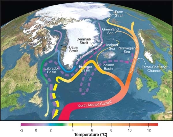
RECOVERY FROM THE LIA AS SEEN IN THE CENTRAL ENGLAND TEMPERATURES 

RELATED POST: [SUPERSTITION, CONFIRMATION BIAS. & CLIMATE CHANGE]

The climate history of Europe records the so called Medieval Warm Period (MWP) that peaked in the period 900-1200 AD at about 0.8C warmer than the average for the millennium that preceded it. Soon thereafter, Europe plunged into a period of global cooling 1303-1860 AD at about 1C cooler than the Medieval Warm Period. It is thought that the cooling was initiated by aerosols from a large scale global volcanism event (see bibliography below and related post on aerosols [LINK] ).

This cold period, known as the Little Ice Age (LIA), was a period of great hardship for Europeans. Canals and rivers were frozen, growth of sea ice around Iceland closed down harbors and shipping, hailstorms and snowstorms were heavy and frequent, and road and water transport was made difficult or impossible. Agricultural failure and consequent starvation and death devastated Europe. The Scandinavian colonies in Greenland starved to death and disappeared (Matthews/Briffa, 2005) (Soon/Baliunas, 2003).

To the Europeans of the time used to relative warmth and agricultural wealth, these extreme weather events seemed abnormal, unusual and bizarre and therefore likely to have evil other-worldly causes and explanations. The human tendency to look for cause and effect relationships in extreme weather predicament and their usual solutions (Maller, 1933), drove the LIA Europeans to climate action not unlike the sorcery killings of Melanesia described in a related post [LINK] .

LIA BIBLIOGRAPHY

1. 1985: Whittington, Graeme. “The little ice age and Scotland’s weather.” Scottish Geographical Magazine 101.3 (1985): 174-178. Some 10,000 years ago with the disappearance of the last Devensian ice, the climate of the British Isles began a slow but general warming. This continued until the middle of the fifteenth century when the Little Ice Age developed, ushering in several centuries of colder weather and violent fluctuations in weather associated with the expansion of the circumpolar vortex. Detailed information of the effect on Scotland’s weather of this major climatic disturbance is rare but The Chronicle of Fifewritten in the seventeenth century by John Lamont does provide some remarkable insights.
2. 1986: Thompson, Lonnie G., et al. “The Little Ice Age as recorded in the stratigraphy of the tropical Quelccaya ice cap.” Science234.4774 (1986): 361-364. The analyses of two ice cores from a southern tropical ice cap provide a record of climatic conditions over 1000 years for a region where other proxy records are nearly absent. Annual variations in visible dust layers, oxygen isotopes, microparticle concentrations, conductivity, and identification of the historical (A.D. 1600) Huaynaputina ash permit accurate dating and time-scale verification. The fact that the Little Ice Age (about A.D. 1500 to 1900) stands out as a significant climatic event in the oxygen isotope and electrical conductivity records confirms the worldwide character of this event.
3. 1990: Clark, James S. “Fire and climate change during the last 750 yr in northwestern Minnesota.” Ecological Monographs 60.2 (1990): 135-159. Charcoal stratigraphic analysis and fire scars on red pine (Pinus resinosa) trees were used to determine spatial and temporal occurrence of fire in 1 km² of old—growth mixed conifer/hardwood forests in northwestern Minnesota. Charcoal was analyzed year by year on petrographic thin sections from annually laminated sediments of three small (≤5 ha) lakes having adjacent catchments. Dated fire scars (n = 150) from recent treefalls provided an independent record of the spatial patterns of past burns. Sedimentology of the varved sediments, water—balance models that use 150 yr of instrumental temperature and precipitation data, and published data were used to identify climate changes in separate studies, and they were used in this study to examine the possible connection between changing fire regimes and climate change. Fire—history data were used to show the changing probability of fire with time since the last fire and the effects of spatial variance (slope and aspect) on the distribution of fires through time. Over the last 750 yr, fire was most frequent (8.6 ± 2.9—yr intervals) during the warm/dry 15th and 16th centuries. Intervals were longer (13.2 ± 8.0 yr) during cooler/moister times from AD 1240 to 1440 and since 1600 (the Little Ice Age). The fire regime during the Little Ice Age consisted of periods during the mid—18th and mid—19th centuries characterized by longer fire intervals of 24.5 ± 10.4 and 43.6 ± 15.9 yr, respectively, and short—term warm/dry periods from 1770 to 1820 and 1870 to 1920 when intervals were 17.9 ± 10.6 and 12.7 ± 10.1, respectively. The probability of fire increased through time, probably in step with fuel accumulation. South— and west—facing slopes burned more frequently than did north and east aspects. Fire suppression began in 1910. During warm periods, probability of fire was sufficiently high that a continuous litter layer was all that was necessary for fire to spread and scar trees. During cool and moist times fire was most likely to occur in years with higher moisture deficits. The combined methods for fire—history analysis provided a more detailed spatial and temporal documentation of fire regimes than has previously been possible from analysis of fire scars or of charcoal counts derived from fossil pollen preparations. Results support predictions of particle—motion physics that thin sections record a local fire history. Because climate varies continuously, the responsiveness of disturbance regime to short— and long—term climatic change suggests caution in the interpretation of fire frequencies that derive from space/time analogies or extrapolation from short—term data.
4. 1993: Bradley, Raymond S., and Philip D. Jonest. “‘Little Ice Age’summer temperature variations: their nature and relevance to recent global warming trends.” The Holocene 3.4 (1993): 367-376. Climatic changes resulting from greenhouse gases will be superimposed on natural climatic variations. High-resolution proxy records of past climate can be used to extend our perspective on regional and hemispheric changes of climate back in time by several hundred years. Using historical, tree-ring and ice core data, we examine climatic variations during the period commonly called the ‘Little Ice Age’. The coldest conditions of the last 560 years were between AD 1570 and 1730, and in the nineteenth century. Unusually warm conditions have prevailed since the 1920s, probably related to a relative absence of major explosive volcanic eruptions and higher levels of greenhouse gases.
5. 1995: Behringer, Wolfgang. “Weather, hunger and fear: Origins of the European Witch Hunts in Climate, Society and Mentality.” German History 13.1 (1995)LINK: LINK TO PDF OF BEHRINGER 1995
6. 1996: Rumsby, Barbara T., and Mark G. Macklin. “River response to the last neoglacial (the ‘Little Ice Age’) in northern, western and central Europe.” Geological Society, London, Special Publications 115.1 (1996): 217-233. Climate changes since AD 1200 have been of high magnitude. Significant lowering of temperatures occurred during the neoglacial (‘Little Ice Age’), between AD 1200–1400 and AD 1600–1800 with maximum cooling in the mid-late eighteenth century. At this time many European valley/cirque glaciers reached their maximum extent since the late Pleistocene. Neoglaciation was followed by an overall warming trend, although with significant reversals superimposed. Alongside these temperature changes were variations in the nature and amount of precipitation, and in consequence, river basins in north, west and central Europe experienced enhanced fluvial activity between 1250 and 1550 and particularly between 1750 and 1900. These phases coincide with periods of climatic transition; cooling after the Medieval optimum and warming during the latter stages of the Little Ice Age respectively. In contrast, the intervening period (1550–1750), which corresponds with the most severe phases of the last neoglacial, was associated with lower rates of fluvial activity.
7. 1996: Keigwin, Lloyd D. “The little ice age and medieval warm period in the Sargasso Sea.” Science (1996): 1504-1508. Sea surface temperature (SST), salinity, and flux of terrigenous material oscillated on millennial time scales in the Pleistocene North Atlantic, but there are few records of Holocene variability. Because of high rates of sediment accumulation, Holocene oscillations are well documented in the northern Sargasso Sea. Results from a radiocarbondated box core show that SST was ∼1°C cooler than today ∼400 years ago (the Little Ice Age) and 1700 years ago, and ∼1°C warmer than today 1000 years ago (the Medieval Warm Period). Thus, at least some of the warming since the Little Ice Age appears to be part of a natural oscillation.
8. 1997: Overpeck, Jonathan, et al. “Arctic environmental change of the last four centuries.” science 278.5341 (1997): 1251-1256. A compilation of paleoclimate records from lake sediments, trees, glaciers, and marine sediments provides a view of circum-Arctic environmental variability over the last 400 years. From 1840 to the mid-20th century, the Arctic warmed to the highest temperatures in four centuries. This warming ended the Little Ice Age in the Arctic and has caused retreats of glaciers, melting of permafrost and sea ice, and alteration of terrestrial and lake ecosystems. Although warming, particularly after 1920, was likely caused by increases in atmospheric trace gases, the initiation of the warming in the mid-19th century suggests that increased solar irradiance, decreased volcanic activity, and feedbacks internal to the climate system played roles.
9. 1998: Fischer, Hubertus, et al. “Little ice age clearly recorded in northern Greenland ice cores.” Geophysical Research Letters25.10 (1998): 1749-1752. Four ice cores drilled in the little investigated area of northern and northeastern Greenland were evaluated for their isotopic (δ¹⁸O) and chemical content. From these rather uniform records a stable isotope temperature time series covering the last 500 years has been deduced, which reveals distinct climate cooling during the 17th and the first half of the 19th century. Timing of the preindustrial temperature deviations agrees well with other northern hemisphere temperature reconstructions, however, their extent (∼1°C) significantly exceeds both continental records as well as previous southern and central Greenland ice core time series. A 20–30% increase in the sea salt aerosol load during these periods supports accompanying circulation changes over the North Atlantic. Comparison with records of potential natural climate driving forces points to an important role of the long‐term solar influence but to only episodically relevant cooling during years directly following major volcano eruptions.
10. 1999: Lean, Judith, and David Rind. “Evaluating sun–climate relationships since the Little Ice Age.” Journal of Atmospheric and Solar-Terrestrial Physics 61.1-2 (1999): 25-36. From the coldest period of the Little Ice Age to the present time, the surface temperature of the Earth increased by perhaps 0.8°C. Solar variability may account for part of this warming which, during the past 350 years, generally tracks fluctuating solar activity levels. While increases in greenhouse gas concentrations are widely assumed to be the primary cause of recent climate change, surface temperatures nevertheless varied significantly during pre-industrial periods, under minimal levels of greenhouse gas variations. A climate forcing of 0.3 W m⁻² arising from a speculated 0.13% solar irradiance increase can account for the 0.3°C surface warming evident in the paleoclimate record from 1650 to 1790, assuming that climate sensitivity is 1°C W⁻¹ m⁻² (which is within the IPCC range). The empirical Sun–climate relationship defined by these pre-industrial data suggests that solar variability may have contributed 0.25°C of the 0.6°C subsequent warming from 1900 to 1990, a scenario which time dependent GCM simulations replicate when forced with reconstructed solar irradiance. Thus, while solar variability likely played a dominant role in modulating climate during the Little Ice Age prior to 1850, its influence since 1900 has become an increasingly less significant component of climate change in the industrial epoch. It is unlikely that Sun–climate relationships can account for much of the warming since 1970, not withstanding recent attempts to deduce long term solar irradiance fluctuations from the observational data base, which has notable occurrences of instrumental drifts. Empirical evidence suggests that Sun–climate relationships exist on decadal as well as centennial time scales, but present sensitivities of the climate system are insufficient to explain these short-term relationships. Still to be simulated over the time scale of the Little Ice Age to the present is the combined effect of direct radiative forcing, indirect forcing via solar-induced ozone changes in the atmosphere, and speculated charged particle mechanisms whose pathways and sensitivities are not yet specified.
11. 1999: Behringer, Wolfgang. “Climatic change and witch-hunting: the impact of the Little Ice Age on mentalities.” Climatic Change43.1 (1999): 335-351. In addition to objective climatic data, subjective or social reactions can also serve as indicators in the assessment of climatic changes. Concerning the Little Ice Age the conception of witchcraft is of enormous importance. Weather-making counts among the traditional abilities of witches. During the late 14^th and 15^th centuries the traditional conception of witchcraft was transformed into the idea of a great conspiracy of witches, to explain “unnatural” climatic phenomena. Because of their dangerous nature, particularly their ability to generate hailstorms, the very idea of witches was the subject of controversial discussion around 1500. The beginnings of meteorology and its emphasis of “natural” reasons in relationship to the development of weather must be seen against the background of this demoniacal discussion. The resurgence of the Little Ice Age revealed the susceptibility of society. Scapegoat reactions may be observed by the early 1560s even though climatologists, thus far, have been of the opinion that the cooling period did not begin until 1565. Despite attempts of containment, such as the calvinistic doctrine of predestination, extended witch-hunts took place at the various peaks of the Little Ice Age because a part of society held the witches directly responsible for the high frequency of climatic anomalies and the impacts thereof. The enormous tensions created in society as a result of the persecution of witches demonstrate how dangerous it is to discuss climatic change under the aspects of morality.
12. 1999: Free, Melissa, and Alan Robock. “Global warming in the context of the Little Ice Age.” Journal of Geophysical Research: Atmospheres 104.D16 (1999): 19057-19070. Understanding the role of volcanic and solar variations in climate change is important not only for understanding the Little Ice Age but also for understanding and predicting the effects of anthropogenic changes in atmospheric composition in the twentieth century and beyond. To evaluate the significance of solar and volcanic effects, we use four solar reconstructions and three volcanic indices as forcings to an energy‐balance model and compare the results with temperature reconstructions. Our use of a model representing the climate system response to solar and volcanic forcings distinguishes this from previous direct comparisons of forcings with temperature series for the Little Ice Age. Use of the model allows us to assess the effects of the ocean heat capacity on the evolution of the temperature response. Using a middle‐of‐the‐road model sensitivity of 3°C for doubled CO₂, solar forcings of less than 0.5% are too small to account for the cooling of the Little Ice Age. Volcanic forcings, in contrast, give climate responses comparable in amplitude to the changes of the Little Ice Age. A combination of solar and volcanic forcings explains much of the Little Ice Age climate change, but these factors alone cannot explain the warming of the twentieth century. The best simulations of the period since 1850 include anthropogenic, solar, and volcanic forcings.
13. 1999: Bond, Gerard C., et al. “The North Atlantic’s 1‐2 kyr climate rhythm: relation to Heinrich events, Dansgaard/Oeschger cycles and the Little Ice Age.” Mechanisms of global climate change at millennial time scales 112 (1999): 35-58. New evidence from deep-sea sediment cores in the subpolar North Atlantic demonstrates that a significant component of sub-Milankovitch climate variability occurs in distinct 1-2 kyr cycles. We have traced that cyclicity from the present to within marine isotope stage 5, an interval spanning more than 80 kyrs. The most robust indicators of the cycle are repeated increases in the percentages of two petrologic tracers, Icelandic glass and hematite-stained grains. Both are sensitive measures of ice rafting episodes associated with ocean surface coolings. The petrologic tracers exhibit a consistent relation to Heinrich events, implying that mechanisms forcing Heinrich events were closely linked to those forcing the cyclicity. Our records further suggest that Dansgaard/Oeschger events may be amplifications of the cycle brought about by the impact of iceberg (fresh water) discharges on North Atlantic thermohaline circulation. The tendency of thermohaline circulation to undergo threshold behavior only when fresh water input is relatively large may explain the absence of Dansgaard/Oeschger events in the Holocene and their long pacings (thousands of years) in the early part of the glaciation. Finally, evidence from cores near Newfoundland confirms previous suggestions that the Little Ice Age was the most recent cold phase of the 1-2 kyr cycle and that the North Atlantic tended to oscillate in a muted Dansgaard/Oeschger-like mode during the Holocene.
14. 1999: Pfister, Christian, and Rudolf Brázdil. “Climatic variability in sixteenth-century Europe and its social dimension: a synthesis.” Climatic Variability in Sixteenth-Century Europe and Its Social Dimension. Springer, Dordrecht, 1999. 5-53.

    The introductory paper to this special issue of Climatic Change summarizes the results of an array of studies dealing with the reconstruction of climatic trends and anomalies in sixteenth-century Europe and their impact on the natural and the social world. Areas discussed include glacier expansion in the Alps, the frequency of natural hazards (floods in central and southern Europe and storms on the Dutch North Sea coast), the impact of climate deterioration on grain prices and wine production, and finally, witch-hunts. The documentary data used for the reconstruction of seasonal and annual precipitation and temperatures in central Europe (Germany, Switzerland and the Czech Republic) include narrative sources, several types of proxy data and 32 weather diaries. Results were compared with long-term composite tree ring series and tested statistically by cross-correlating series of indices based on documentary data from the sixteenth century with those of simulated indices based on instrumental series (1901–1960). It was shown that series of indices can be taken as good substitutes for instrumental measurements. A corresponding set of weighted seasonal and annual series of temperature and precipitation indices for central Europe was computed from series of temperature and precipitation indices for Germany, Switzerland and the Czech Republic, the weights being in proportion to the area of each country. The series of central European indices were then used to assess temperature and precipitation anomalies for the 1901–1960 period using transfer functions obtained from instrumental records. The statistical analysis of these series of estimated temperature and precipitation anomalies yielded features which are similar to those obtained from instrumental series. Results show that winter temperatures remained below the 1901–1960 average except in the 1520s and 1550s. Springs fluctuated from 0.3°C to 0.8°C below this average. Summer climate was divided into three periods of almost equal length. The first was characterized by an alternation of cool and warmer seasons. The second interval was 0.3°C warmer and between 5 and 6% drier than in the 1901–1960 period. It is emphasized that this warm period included several cold extremes in contrast to the recent period of warming. Summers from 1560 were 0.4°C colder and 4% more humid. Autumns were 0.7°C colder in the 1510s and 20% wetter in the 1570s. The deterioration of summer climate in the late sixteenth century initiated a second period of enlarged glaciers in this millennium (the first having been in the fourteenth century) which did not end until the late nineteenth century. An analysis of forcing factors (solar, volcanic, ENSO, greenhouse) points only to some volcanic forcing. In order to understand circulation patterns in the sixteenth century in terms of synoptic climatology, proxy information was mapped for a number of anomalous months. Attempts to compare circulation patterns in the sixteenth century with twentieth-century analogues revealed that despite broad agreements in pressure patterns, winters with distinct northeasterly patterns were more frequent in the sixteenth century, whereas the declining summer temperatures from the mid-1560s seem to be associated with a decreasing frequency of anticyclonic ridging from the Azores’ center of action towards continental Europe. The number of severe stonns on the Dutch North Sea coast was four times greater in the second half of the century than in the first. A more or less continuous increase in the number of floods over the entire century occurred in Germany and the Czech lands. The Iberian peninsula and the Garonne basin (France) had the greatest number of severe floods in the 1590s. The analysis of the effects of climate on rye prices in four German towns involved a model that included monthly temperatures and precipitation values known to affect grain production. The correlation with rye prices was found significant for the entire century and reached its highest values between 1565 and 1600. From the 1580s to the turn of the century wine production slumped almost simultaneously in four regions over a distance of 800 kilometers (Lake Zurich to western Hungary). This had far-reaching consequences for the Habsburg treasury and promoted a temporary shift in drinking habits from wine to beer. Peasant communities which were suffering large collective damage from the effects of climatic change pressed authorities for the organization of witch-hunts. Seemingly most witches were burnt as scapegoats of climatic change.

15. 2000: Luckman, Brian H. “The little ice age in the Canadian Rockies.” Geomorphology 32.3-4 (2000): 357-384. This paper reviews the evidence and history of glacier fluctuations during the Little Ice Age (LIA) in the Canadian Rockies. Episodes of synchronous glacier advance occurred in the 12th–13th, early 18th and throughout the 19th centuries. Regional ice cover was probably greatest in the mid-19th century, although in places the early 18th century advance was more extensive. Glaciers have lost over 25% of their area in the 20th century. Selective preservation of the glacier record furnishes an incomplete chronology of events through the 14th–17th centuries. In contrast, varve sequences provide continuous, annually resolved records of sediments for at least the last millennium in some highly glacierized catchments. Such records have been used to infer glacier fluctuations. Evaluation of recent proxy climate reconstructions derived from tree-rings provides independent evidence of climate fluctuations over the last millennium. Most regional glacier advances follow periods of reduced summer temperatures, reconstructed from tree rings particularly ca. 1190–1250, 1280–1340, 1690s and the 1800s. Reconstructed periods of higher precipitation at Banff, Alberta since 1500 are 1515–1550, 1585–1610, 1660–1680 and the 1880s. Glacier advances in the early 1700s, the late 1800s and, in places, the 1950–1970s reflect both increased precipitation and reduced summer temperatures. Negative glacier mass balances from 1976 to 1995 were caused by decreased winter balances. The glacier fluctuation record does not contain a simple climate signal: it is a complex response to several interacting factors that operate at different timescales. Evaluation of climate proxies over the last millennium indicates continuous variability at several superimposed timescales, dominated by decade–century patterns. Only the 19th century shows a long interval of sustained cold summers. This suggests that simplistic concepts of climate over this period should be abandoned and replaced with more realistic records based on continuous proxy data series. The use of the term LIA should be restricted to describing a period of extended glacier cover rather than being used to define a period with specific climate conditions.
16. 2000: Reiter, Paul. “From Shakespeare to Defoe: malaria in England in the Little Ice Age.” Emerging infectious diseases 6.1 (2000): Present global temperatures are in a warming phase that began 200 to 300 years ago. Some climate models suggest that human activities may have exacerbated this phase by raising the atmospheric concentration of carbon dioxide and other greenhouse gases. Discussions of the potential effects of the weather include predictions that malaria will emerge from the tropics and become established in Europe and North America. The complex ecology and transmission dynamics of the disease, as well as accounts of its early history, refute such predictions. Until the second half of the 20th century, malaria was endemic and widespread in many temperate regions, with major epidemics as far north as the Arctic Circle. From 1564 to the 1730s the coldest period of the Little Ice Age malaria was an important cause of illness and death in several parts of England. Transmission began to decline only in the 19th century, when the present warming trend was well under way. The history of the disease in England underscores the role of factors other than temperature in malaria transmission.
17. 2001: Ogilvie, Astrid EJ, and Trausti Jónsson. “” Little ice age” research: A perspective from Iceland.” Climatic Change 48.1 (2001): 9-52. The development during the nineteenth and twentieth centuries of the sciences of meteorology and climatology and their subdisciplines has made possible an ever-increasing understanding of the climate of the past. In particular, the refinement of palaeoclimatic proxy data has meant that the climate of the past thousand years has begun to be extensively studied. In the context of this research, it has often been suggested that a warm epoch occurred in much of northern Europe, the north Atlantic, and other parts of the world, from around the ninth through the fourteenth centuries, and that this was followed by a decline in temperatures culminating in a “Little Ice Age” from about 1550 to 1850 (see e.g. Lamb, 1965, 1977; Flohn, 1978). The appelations “Medieval Warm Period” and “Little Ice Age” have entered the literature and are frequently used without clear definition. More recently, however, these terms have come under closer scrutiny (see, e.g. Ogilvie, 1991, 1992; Bradley and Jones, 1992; Mikami, 1992; Briffa and Jones, 1993; Bradley and Jones, 1993; Hughes and Diaz, 1994; Jones et al., 1998; Mann et al., 1999; Crowley and Lowery, 2000). As research continues into climatic fluctuations over the last 1000 to 2000 years, a pattern is emerging which suggests a far more complex picture than early research into the history of climate suggested. In this paper, the origins of the term “Little Ice Age” are considered. Because of the emphasis on the North Atlantic in this volume, the prime focus is on research that has been undertaken in this region, with a perspective on the historiography of historical climatology in Iceland as well as on the twentieth-century climate of Iceland. The phrase “Little Ice Age” has become part of the scientific and popular thinking on the climate of the past thousand years. However, as knowledge of the climate of the Holocene continues to grow, the term now seems to cloud rather than clarify thinking on the climate of the past thousand years. It is hoped that the discussion here will encourage future researchers to focus their thinking on exactly and precisely what is meant when the term “Little Ice Age” is used.
18. 2001: Grove, Jean M. “The initiation of the” Little Ice Age” in regions round the North Atlantic.” Climatic change 48.1 (2001): 53-82. The “Little Ice Age” was the most recent period during which glaciers extended globally, their fronts oscillating about advanced positions. It is frequently taken as having started in the sixteenth or seventeenth century and ending somewhere between 1850 and 1890, but Porter (1981) pointed out that the “Little Ice Age” may ‘have begun at least three centuries earlier in the North Atlantic region than is generally inferred’. The glacial fluctuations of the last millennium have been traced in the greatest detail in the Swiss Alps, where the “Little Ice Age” is now seen as starting with advances in the thirteenth century, and reaching an initial culmination in the fourteenth century. In the discussion here, evidence from Canada, Greenland, Iceland, Spitsbergen and Scandinavia is compared with that from Switzerland. Such comparisons have been facilitated by improved methods of calibrating radiocarbon dates to calendar dates and by increasing availability of evidence revealed during the current retreat phase. It is concluded that the “Little Ice Age” was initiated before the early fourteenth century in regions surrounding the North Atlantic.
19. 2002: Hendy, Erica J., et al. “Abrupt decrease in tropical Pacific sea surface salinity at end of Little Ice Age.” Science 295.5559 (2002): 1511-1514. A 420-year history of strontium/calcium, uranium/calcium, and oxygen isotope ratios in eight coral cores from the Great Barrier Reef, Australia, indicates that sea surface temperature and salinity were higher in the 18th century than in the 20th century. An abrupt freshening after 1870 occurred simultaneously throughout the southwestern Pacific, coinciding with cooling tropical temperatures. Higher salinities between 1565 and 1870 are best explained by a combination of advection and wind-induced evaporation resulting from a strong latitudinal temperature gradient and intensified circulation. The global Little Ice Age glacial expansion may have been driven, in part, by greater poleward transport of water vapor from the tropical Pacific
20. 2002: Mann, Michael E. “Little ice age.” Encyclopedia of global environmental change 1 (2002): 504-509. The term Little Ice Age is reserved for the most extensive recent period of mountain glacier expansion and is conventionally defined as the 16th–mid 19th century period during which European climate was most strongly impacted. This period begins with a trend towards enhanced glacial
    conditions in Europe following the warmer conditions of the so-called medieval warm period or medieval climatic optimum of Europe (see Medieval Climatic Optimum, Volume 1), and terminates with the dramatic retreat of these glaciers during the 20th century. While there is evidence that many other regions outside Europe exhibited periods of cooler conditions, expanded glaciation, and significantly altered climate conditions, the timing and nature of these variations are highly variable from region to region, and the notion of the Little Ice Age as a globally synchronous cold period has all but been dismissed (Bradley and Jones, 1993; Mann et al., 1999). If defined as a large-scale event, the Little Ice Age must instead be considered a time of modest cooling of the Northern Hemisphere, with temperatures dropping by about 0.6 °C during the 15th–19th
21. 2003: Nesje, Atle, and Svein Olaf Dahl. “The ‘Little Ice Age’–only temperature?.” The Holocene 13.1 (2003): 139-145. Understanding the climate of the last few centuries, including the ‘Little Ice Age’, may help us better understand modern-day natural climate variability and make climate predictions. The conventional view of the climate development during the last millennium has been that it followed the simple sequence of a ‘Mediaeval Warm Period’, a cool ‘Little Ice Age’ followed by warming in the later part of the nineteenth century and during the twentieth century. This view was mainly based on evidence from western Europe and the North Atlantic region. Recent research has, however, challenged this rather simple sequence of climate development in the recent past. Data presented here indicate that the rapid glacier advance in the early eighteenth century in southern Norway was mainly due to increased winter precipitation: mild, wet winters due to prevailing ‘positive North Atlantic Oscillation (NAO) weather mode’ in the first half of the eighteenth century; and not only lower summer temperatures. A comparison of recent mass-balance records and ‘Little Ice Age’ glacier fluctuations in southern Norway and the European Alps suggests that the asynchronous ‘Little Ice Age’ maxima in the two regions may be attributed to multidecadal trends in the north–south dipole NAO pattern.
22. 2004: Oster, Emily. “Witchcraft, weather and economic growth in Renaissance Europe.” Journal of Economic Perspectives 18.1 (2004): 215-228. between the thirteenth and nineteenth centuries, as many as one million individuals in Europe were executed for the crime of witchcraft. The majority of the trials and executions took place during the sixteenth and seventeenth centuries. During this period, the speed and volume of executions were astonishing: in one German town, as many as 400 people were killed in a single day (Midelfort, 1972). The trials were ubiquitous: conducted by both ecclesiastical and secular courts; by both Catholics and Protestants. The victims were primarily women, primarily poor and disproportionately widows. The persecutions took place throughout Europe, starting and ending earlier in southwest Europe than in the northern and eastern areas, and spread even across the Atlantic Ocean to Salem, Massachusetts. Although witchcraft trials in Europe and America largely ended by the late eighteenth century, witchcraft accusations and killings still take place in many countries today, particularly in the developing world. For example, witchcraft is often blamed for AIDS deaths in sub-Saharan Africa (Ashforth, 2001), and Miguel (2003) shows that negative economic shocks are associated with increases in witch killing in modern Tanzania. Belief in the witch, and fear of her, is enduring. While much work has been done on the motivations behind the European trials, the large-scale causes remain unknown. The existing work has primarily been concerned with the factors that played into trials on a small scale—why a certain individual was targeted or why a certain type of individual was targeted in a given area. This work has indicated that there was a diverse set of issues that played into trials on an individual level. More broadly, however, there are few causal explanations
    for why witchcraft trials happened at all and on such a large scale in so many
    y Emily Oster is a Ph.D. student in economics, Harvard University, Cambridge, Massachusetts. Her e-mail address is eoster@post.harvard.edu. Journal of Economic Perspectives—Volume 18, Number 1—Winter 2004—Pages 215–228 areas at the times that they did. The earliest trials, going back to the thirteenth century, were the work of church institutions, particularly the Catholic Inquisition, but the mass of trials later in the period saw very little formal church involvement of this type. Various hypotheses have been offered: for example, a need by the male medical profession to rid the world of midwives and female folk healers (Ehrenreich and English, 1973); a perceived need for moral boundaries by the Catholic church (Ben-Yehuda, 1980); or an increase in syphilis and subsequent increase in the mentally ill, who were then targeted as witches (Ross, 1995). This paper explores the possibility that the witchcraft trials are a large-scale example of violence and scapegoating prompted by a deterioration in economic conditions. In this case, the downturn was brought on by a decrease in temperature and resulting food shortages. The most active period of the witchcraft trials coincides with a period of lower than average temperature known to climatologists as the “little ice age.” The colder temperatures increased the frequency of crop failure, and colder seas prevented cod and other fish from migrating as far north, eliminating this vital food source for some northern areas of Europe (Fagan, 2000). Several kinds of data show more than a coincidental relationship between witch trials, weather and economic growth. In a time period when the reasons for changes in weather were largely a mystery, people would have searched for a scapegoat in the face of deadly changes in weather patterns. “Witches” became target for blame because there was an existing cultural framework that both allowed their persecution and suggested that they could control the weather. Background on Witchcraft and the Little Ice Age
23. 2005: Matthews, John A., and Keith R. Briffa. “The ‘Little Ice Age’: re‐evaluation of an evolving concept.” Geografiska Annaler: Series A, Physical Geography 87.1 (2005): 17-36. This review focuses on the development of the ‘Little Ice Age’ as a glaciological and climatic concept, and evaluates its current usefulness in the light of new data on the glacier and climatic variations of the last millennium and of the Holocene. ‘Little Ice Age’ glacierization occurred over about 650 years and can be defined most precisely in the European Alps (c. AD 1300–1950) when extended glaciers were larger than before or since. ‘Little Ice Age’ climate is defined as a shorter time interval of about 330 years (c. AD 1570–1900) when Northern Hemisphere summer temperatures (land areas north of 20°N) fell significantly below the AD 1961–1990 mean. This climatic definition overlaps the times when the Alpine glaciers attained their latest two highstands (AD 1650 and 1850). It is emphasized, however, that ‘Little Ice Age’ glacierization was highly dependent on winter precipitation and that ‘Little Ice Age’ climate was not simply a matter of summer temperatures. Both the glacier‐centred and the climate‐centred concepts necessarily encompass considerable spatial and temporal variability, which are investigated using maps of mean summer temperature variations over the Northern Hemisphere at 30‐year intervals from AD 1571 to 1900. ‘Little Ice Age’‐type events occurred earlier in the Holocene as exemplified by at least seven glacier expansion episodes that have been identified in southern Norway. Such events provide a broader context and renewed relevance for the ‘Little Ice Age’, which may be viewed as a ‘modern analogue’ for the earlier events; and the likelihood that similar events will occur in the future has implications for climatic change in the twenty‐first century. It is concluded that the concept of a ‘Little Ice Age’ will remain useful only by (1) continuing to incorporate the temporal and spatial complexities of glacier and climatic variations as they become better known, and (2) by reflecting improved understanding of the Earth‐atmosphere‐ocean system and its forcing factors through the interaction of palaeoclimatic reconstruction with climate modelling.
24. 2005: Brázdil, Rudolf, et al. “Historical climatology in Europe–the state of the art.” Climatic change 70.3 (2005): 363-430. This paper discusses the state of European research in historical climatology. This field of science and an overview of its development are described in detail. Special attention is given to the documentary evidence used for data sources, including its drawbacks and advantages. Further, methods and significant results of historical-climatological research, mainly achieved since 1990, are presented. The main focus concentrates on data, methods, definitions of the “Medieval Warm Period” and the “Little Ice Age”, synoptic interpretation of past climates, climatic anomalies and natural disasters, and the vulnerability of economies and societies to climate as well as images and social representations of past weather and climate. The potential of historical climatology for climate modelling research is discussed briefly. Research perspectives in historical climatology are formulated with reference to data, methods, interdisciplinarity and impacts.
25. 2006: Bräuning, Achim. “Tree-ring evidence of ‘Little Ice Age’glacier advances in southern Tibet.” The Holocene 16.3 (2006): 369-380. The history of late Holocene glacier fluctuations in eastern Tibet was studied by determining the ages of trees growing on glacier deposits. Maximum tree ages yield minimum ages of AD 1760 and 1780 for moraine formation at the maximum extent of the ‘Little Ice Age’ glacier advances in two glacier forefields. Subsequent moraines could be dated to the beginning of the nineteenth and the beginning of the twentieth century. Larch trees from a third glacier forefield in southeastern Tibet show evidence of glacier activity from 1580 to 1590, from the end of the eighteenth to the beginning of the nineteenth century and from 1860 to 1880. One glacier at Mt Gyalaperi recently advanced in both 1951 and 1987. Periods of glacier advances can partly be correlated with periods of growth reductions in chronologies of total ring width and maximum latewood density derived from trees growing on slopes above the glacier valleys. Correlation functions with meteorological data suggest that maximum latewood density of subalpine Picea balfouriana, Larix griffithii and Abies delavayi var.motouensis is positively correlated with summer temperature, while ring width of these species and of subalpine Juniperus tibetica is also sensitive to winter conditions prior to the growing season.
26. 2006: Pfister, Christian. “Climatic extremes, recurrent crises and witch hunts: strategies of European societies in coping with exogenous shocks in the late sixteenth and early seventeenth centuries.” The Medieval History Journal 10.1-2 (2006): 33-73. In the late sixteenth and early seventeenth centuries, continental Europe north of the Alps was afflicted by a 13-year cycle of frequent cold and rainy summers which was the result of a series of volcanic explosions in the tropics. The inclement weather led to recurrent subsistence crises and to multiple floods in the Alps following from extensive glacier advances. This article discusses the relationship between ‘climate’ and ‘history’ from the example of this unique period. The vulnerability of food production in Europe to climatic hazard is assessed from an impact model. The result shows that the period 1560 to 1630 is most prominently marked by a high level of climatic stress. Likewise, this study demonstrates how authorities in Val Aosta (Italy) responded to annually recurrent floods in the 1590s triggered by the advancing Ruitor glacier. Finally, by confirming the thesis advanced by Wolfgang Behringer relating extensive witch hunts during that period to climatic change and recurrent subsistence crises, this article makes a plea for bridging the gap separating studies of climate from those of culture.
27. 2006: Pfister, Christian, and Rudolf Brázdil. “Social vulnerability to climate in the” Little Ice Age“: an example from Central Europe in the early 1770s.” Climate of the Past 2.2 (2006): 115-129. The paper is oriented on social vulnerability to climate in Switzerland and in the Czech Lands during the early 1770s. Documentary sources of climate related to man-made archives are discussed. Methods of temperature and precipitation reconstruction based on this evidence as well as climate impact analyses are presented. Modelling of Little Ice Age-type Impacts (LIATIMP) is applied to highlight climate impacts during the period 1750?1800 in the Swiss Plateau and in the Czech Lands. LIATIMP are defined as adverse climate situations affecting agricultural production, mainly in terms of rainy autumns, cold springs and rainy harvest-periods. The most adverse weather patterns according to this model occurred from 1769 to 1771 causing two, in the case of the Czech Lands even three successive harvest failures. The paper addresses the social and economic consequences of this accumulation of climatic stress and explores how the authorities and the victims dealt with this situation.
28. 2008: Crowley, Thomas J., et al. “Volcanism and the little ice age.” PAGES news 16.2 (2008): 22-23.  Although solar variability has often been considered the primary agent for LIA cooling, the most comprehensive test of this explanation (Hegerl et al., 2003) points instead to volcanism being substantially more important, explaining as much as 40% of the decadal-scale variance during the LIA. Yet, one problem that has continually plagued climate researchers is that the paleovolcanic record, reconstructed from Antarctic and Greenland ice cores, cannot be well calibrated against the instrumental record. This is because the primary in-strumental volcano reconstruction used by the climate community is that of Sato et al. (1993), which is relatively poorly con-strained by observations prior to 1960 (es-pecially in the southern hemisphere). Here, we report on a new study that has successfully calibrated the Antarctic sulfate record of volcanism from the 1991 eruptions of Pinatubo (Philippines) and Hudson (Chile) against satellite aerosol op-tical depth (AOD) data (AOD is a measure of stratospheric transparency to incoming solar radiation). A total of 22 cores yield an area-weighted sulfate accumulation rate of 10.5 kg/km2, which translates into a conversion rate for AOD of 0.011 AOD/kg/km2 sulfate. We validated our time series by comparing a canonical growth and decay curve for eruptions for Krakatau (1883), the 1902 Caribbean eruptions (pri marily Santa Maria), and the 1912 eruption of Novarupta/Katmai (Alaska) against a reanalysis (Stothers, 1996) of the original AOD data and lunar eclipse estimates of AOD for Krakatau (Keen, 1983). The agreement (Fig. 1) is very good—essentially within the uncertainty of the independent data. Our new ice core reconstruction shows several significant disagreements with the Sato et al. (1993).
29. 2009: Masiokas, M. H., et al. “Little Ice Age fluctuations of small glaciers in the Monte Fitz Roy and Lago del Desierto areas, south Patagonian Andes, Argentina.” Palaeogeography, Palaeoclimatology, Palaeoecology 281.3-4 (2009): 351-362. Current knowledge about late Holocene glacier fluctuations in the south Patagonian Andes is mainly based on evidence from large outlet glaciers of the North and South Patagonian Icefields, and few data exist for the smaller glaciers elsewhere in the region. Here we provide dendrogeomorphological evidence for Little Ice Age (LIA) and post-LIA activity for five small glaciers near the northeast margin of the South Patagonian Icefield. The study sites include Glaciar Torre and Piedras Blancas in the Monte Fitz Roy area, and three adjacent glaciers near Lago del Desierto. At these sites the LIA maximum position was identified by massive moraines with mature trees dating to the late 1500s–early 1600s. Several older moraines were observed beyond these limits but could not be precisely dated. Relatively synchronous advances occurred at most glaciers in the early 1700s and were dated using living trees and in situ, subfossil material. All glaciers show three to five subsequent advances mostly concentrated between the mid-19th and early 20th centuries. Estimates based on Landsat TM imagery indicate these glaciers lost between 15 and 46% of their LIA areas by 1984 and a further 5–18% by 2005, with the smallest glaciers showing the greatest proportional loss. Paired comparisons of contemporary and the earliest known photography for the glaciers in the Fitz Roy area confirm this mass loss. These results provide important new information on the glacier history of this area but additional, more precisely-dated records are needed from many more sites before we can fully elucidate the complex late Holocene glacial history of this region.
30. 2009: Mann & Zhang. “Global signatures and dynamical origins of the Little Ice Age and Medieval Climate Anomaly.” Science 326.5957 (2009): 1256-1260. Global temperatures are known to have varied over the past 1500 years, but the spatial patterns have remained poorly defined. We used a global climate proxy network to reconstruct surface temperature patterns over this interval. The Medieval period is found to display warmth that matches or exceeds that of the past decade in some regions, but which falls well below recent levels globally. This period is marked by a tendency for La Niña–like conditions in the tropical Pacific. The coldest temperatures of the Little Ice Age are observed over the interval 1400 to 1700 C.E., with greatest cooling over the extratropical Northern Hemisphere continents. The patterns of temperature change imply dynamical responses of climate to natural radiative forcing changes involving El Niño and the North Atlantic Oscillation–Arctic Oscillation.
31. 2010: Dull, Robert A., et al. “The Columbian encounter and the Little Ice Age: Abrupt land use change, fire, and greenhouse forcing.” Annals of the Association of American Geographers100.4 (2010): 755-771. Pre-Columbian farmers of the Neotropical lowlands numbered an estimated 25 million by 1492, with at least 80 percent living within forest biomes. It is now well established that significant areas of Neotropical forests were cleared and burned to facilitate agricultural activities before the arrival of Europeans. Paleoecological and archaeological evidence shows that demographic pressure on forest resources—facilitated by anthropogenic burning—increased steadily throughout the Late Holocene, peaking when Europeans arrived in the late fifteenth century. The introduction of Old World diseases led to recurrent epidemics and resulted in an unprecedented population crash throughout the Neotropics. The rapid demographic collapse was mostly complete by 1650, by which time it is estimated that about 95 percent of all indigenous inhabitants of the region had perished. We review fire history records from throughout the Neotropical lowlands and report new high-resolution charcoal records and demographic estimates that together support the idea that the Neotropical lowlands went from being a net source of CO₂ to the atmosphere before Columbus to a net carbon sink for several centuries following the Columbian encounter. We argue that the regrowth of Neotropical forests following the Columbian encounter led to terrestrial biospheric carbon sequestration on the order of 2 to 5 Pg C, thereby contributing to the well-documented decrease in atmospheric CO₂ recorded in Antarctic ice cores from about 1500 through 1750, a trend previously attributed exclusively to decreases in solar irradiance and an increase in global volcanic activity. We conclude that the post-Columbian carbon sequestration event was a significant forcing mechanism of Little Ice Age cooling.
32. 2011: Bertler, N. A. N., P. A. Mayewski, and L. Carter. “Cold conditions in Antarctica during the Little Ice Age—Implications for abrupt climate change mechanisms.” Earth and Planetary Science Letters 308.1 (2011): 41-51. The Little Ice Age (LIA) is one of the most prominent climate shifts in the past 5000 yrs. It has been suggested that the LIA might be the most recent of the Dansgaard–Oeschger events, which are better known as abrupt, large scale climate oscillations during the last glacial period. If the case, then according to Broecker (2000a, 2000b) Antarctica should have warmed during the LIA, when the Northern Hemisphere was cold. Here we present new data from the Ross Sea, Antarctica, that indicates surface temperatures were ~ 2 °C colder during the LIA, with colder sea surface temperatures in the Southern Ocean and/or increased sea-ice extent, stronger katabatic winds, and decreased snow accumulation. Whilst we find there was large spatial and temporal variability, overall Antarctica was cooler and stormier during the LIA. Although temperatures have warmed since the termination of the LIA, atmospheric circulation strength has remained at the same, elevated level. We conclude, that the LIA was either caused by alternative forcings, or that the sea-saw mechanism operates differently during warm periods.
33. 2011: Morellón, Mario, et al. “Climate changes and human activities recorded in the sediments of Lake Estanya (NE Spain) during the Medieval Warm Period and Little Ice Age.” Journal of Paleolimnology 46.3 (2011): 423-452. A multi-proxy study of short sediment cores recovered in small, karstic Lake Estanya (42°02′ N, 0°32′ E, 670 m.a.s.l.) in the Pre-Pyrenean Ranges (NE Spain) provides a detailed record of the complex environmental, hydrological and anthropogenic interactions occurring in the area since medieval times. The integration of sedimentary facies, elemental and isotopic geochemistry, and biological proxies (diatoms, chironomids and pollen), together with a robust chronological control, provided by AMS radiocarbon dating and ²¹⁰Pb and ¹³⁷Cs radiometric techniques, enabled precise reconstruction of the main phases of environmental change, associated with the Medieval Warm Period (MWP), the Little Ice Age (LIA) and the industrial era. Shallow lake levels and saline conditions with poor development of littoral environments prevailed during medieval times (1150–1300 AD). Generally higher water levels and more dilute waters occurred during the LIA (1300–1850 AD), although this period shows a complex internal paleohydrological structure and is contemporaneous with a gradual increase of farming activity. Maximum lake levels and flooding of the current littoral shelf occurred during the nineteenth century, coinciding with the maximum expansion of agriculture in the area and prior to the last cold phase of the LIA. Finally, declining lake levels during the twentieth century, coinciding with a decrease in human pressure, are associated with warmer climate conditions. A strong link with solar irradiance is suggested by the coherence between periods of more positive water balance and phases of reduced solar activity. Changes in winter precipitation and dominance of NAO negative phases would be responsible for wet LIA conditions in western Mediterranean regions. The main environmental stages recorded in Lake Estanya are consistent with Western Mediterranean continental records, and show similarities with both Central and NE Iberian reconstructions, reflecting a strong climatic control of the hydrological and anthropogenic changes during the last 800 years.
34. 2012: Orsi, Anais J., Bruce D. Cornuelle, and Jeffrey P. Severinghaus. “Little Ice Age cold interval in West Antarctica: evidence from borehole temperature at the West Antarctic Ice Sheet (WAIS) divide.” Geophysical Research Letters 39.9 (2012).  The largest climate anomaly of the last 1000 years in the Northern Hemisphere was the Little Ice Age (LIA) from 1400–1850 C.E., but little is known about the signature of this event in the Southern Hemisphere, especially in Antarctica. We present temperature data from a 300 m borehole at the West Antarctic Ice Sheet (WAIS) Divide. Results show that WAIS Divide was colder than the last 1000‐year average from 1300 to 1800 C.E. The temperature in the time period 1400–1800 C.E. was on average 0.52 ± 0.28°C colder than the last 100‐year average. This amplitude is about half of that seen at Greenland Summit (GRIP). This result is consistent with the idea that the LIA was a global event, probably caused by a change in solar and volcanic forcing, and was not simply a seesaw‐type redistribution of heat between the hemispheres as would be predicted by some ocean‐circulation hypotheses. The difference in the magnitude of the LIA between Greenland and West Antarctica suggests that the feedbacks amplifying the radiative forcing may not operate in the same way in both regions
35. 2012: Nussbaumer, Samuel U., and Heinz J. Zumbühl. “The Little Ice Age history of the Glacier des Bossons (Mont Blanc massif, France): a new high-resolution glacier length curve based on historical documents.” Climatic Change 111.2 (2012): 301-334. Historical and proxy records document that there is a substantial asynchronous development in temperature, precipitation and glacier variations between European regions during the last few centuries. The causes of these temporal anomalies are yet poorly understood. Hence, highly resolved glacier reconstructions based on historical evidence can give valuable insights into past climate, but they exist only for few glaciers worldwide. Here, we present a new reconstruction of length changes for the Glacier des Bossons (Mont Blanc massif, France), based on unevaluated historical material. More than 250 pictorial documents (drawings, paintings, prints, photographs, maps) as well as written accounts have been critically analysed, leading to a revised picture of the glacier’s history, especially from the mid-eighteenth century up to the 1860s. Very important are the drawings by Jean-Antoine Linck, Samuel Birmann and Eugène Viollet-le Duc, which depict meticulously the glacier’s extent during the vast advance and subsequent retreat during the nineteenth century. The new glacier reconstruction extends back to AD 1580 and proves maxima of the Glacier des Bossons around 1610/1643, 1685, 1712, 1777, 1818, 1854, 1892, 1921, 1941, and 1983. The Little Ice Age maximum extent was reached in 1818. Until the present, the glacier has lost about 1.5 km in length, and it is now shorter than at any time during the reconstruction period. The Glacier des Bossons reacts faster than the nearby Mer de Glace (glacier reconstruction back to AD 1570 available). The Mont Blanc area is, together with the valley of Grindelwald in the Swiss Alps (two historical glacier reconstructions available back to AD 1535, and 1590, respectively), among the two regions that are probably best-documented in the world regarding historical glacier data
36. 2012: Miller, Gifford H., et al. “Abrupt onset of the Little Ice Age triggered by volcanism and sustained by sea‐ice/ocean feedbacks.” Geophysical Research Letters 39.2 (2012). Northern Hemisphere summer temperatures over the past 8000 years have been paced by the slow decrease in summer insolation resulting from the precession of the equinoxes. However, the causes of superposed century‐scale cold summer anomalies, of which the Little Ice Age (LIA) is the most extreme, remain debated, largely because the natural forcings are either weak or, in the case of volcanism, short lived. Here we present precisely dated records of ice‐cap growth from Arctic Canada and Iceland showing that LIA summer cold and ice growth began abruptly between 1275 and 1300 AD, followed by a substantial intensification 1430–1455 AD. Intervals of sudden ice growth coincide with two of the most volcanically perturbed half centuries of the past millennium. A transient climate model simulation shows that explosive volcanism produces abrupt summer cooling at these times, and that cold summers can be maintained by sea‐ice/ocean feedbacks long after volcanic aerosols are removed. Our results suggest that the onset of the LIA can be linked to an unusual 50‐year‐long episode with four large sulfur‐rich explosive eruptions, each with global sulfate loading >60 Tg. The persistence of cold summers is best explained by consequent sea‐ice/ocean feedbacks during a hemispheric summer insolation minimum; large changes in solar irradiance are not required.
37. 2013: Kelly, Morgan, and Cormac Ó Gráda. “The waning of the little ice age: climate change in early modern Europe.” Journal of Interdisciplinary History 44.3 (2013): 301-325. The supposed ramifications of the Little Ice Age, a period of cooling temperatures straddling several centuries in northwestern Europe, reach far beyond meteorology into economic, political, and cultural history. The available annual temperature series from the late Middle Ages to the end of the nineteenth century, however, contain no major breaks, cycles, or trends that could be associated with the existence of a Little Ice Age. Furthermore, the series of resonant images, ranging from frost fairs to contracting glaciers and from dwindling vineyards to disappearing Viking colonies, often adduced as effects of a Little Ice Age, can also be explained without resort to climate change.
38. 2013: White, Sam. “The real little ice age.” Journal of Interdisciplinary History 44.3 (2013): 327-352. The Little Ice Age is not a dogma. It is an increasingly firm consensus backed by considerable evidence across a variety of sources. To disprove it, or even to call it into question, would mean finding systematic errors in several types of proxy data. Kelly and Ó Gráda have not cleared any of these hurdles, or even come close. The refutation of their arguments demonstrates just how strong the evidence for the Little Ice Age has become and just how important it is for historians to take it seriously.
39. 2013: Lehner, Flavio, et al. “Amplified inception of European Little Ice Age by sea ice–ocean–atmosphere feedbacks.” Journal of Climate 26.19 (2013): 7586-7602. The inception of the Little Ice Age (~1400–1700 AD) is believed to have been driven by an interplay of external forcing and climate system internal variability. While the hemispheric signal seems to have been dominated by solar irradiance and volcanic eruptions, the understanding of mechanisms shaping the climate on a continental scale is less robust. In an ensemble of transient model simulations and a new type of sensitivity experiments with artificial sea ice growth, the authors identify a sea ice–ocean–atmosphere feedback mechanism that amplifies the Little Ice Age cooling in the North Atlantic–European region and produces the temperature pattern suggested by paleoclimatic reconstructions. Initiated by increasing negative forcing, the Arctic sea ice substantially expands at the beginning of the Little Ice Age. The excess of sea ice is exported to the subpolar North Atlantic, where it melts, thereby weakening convection of the ocean. Consequently, northward ocean heat transport is reduced, reinforcing the expansion of the sea ice and the cooling of the Northern Hemisphere. In the Nordic Seas, sea surface height anomalies cause the oceanic recirculation to strengthen at the expense of the warm Barents Sea inflow, thereby further reinforcing sea ice growth. The absent ocean–atmosphere heat flux in the Barents Sea results in an amplified cooling over Northern Europe. The positive nature of this feedback mechanism enables sea ice to remain in an expanded state for decades up to a century, favoring sustained cold periods over Europe such as the Little Ice Age. Support for the feedback mechanism comes from recent proxy reconstructions around the Nordic Seas.
40. 2013: Schleussner, Carl-Friedrich, and G. Feulner. “A volcanically triggered regime shift in the subpolar North Atlantic Ocean as a possible origin of the Little Ice Age.” Climate of the Past 9.3 (2013). Among the climatological events of the last millennium, the Northern Hemisphere Medieval Climate
    Anomaly succeeded by the Little Ice Age are of exceptional importance. The origin of these regional climate anomalies remains a subject of debate and besides external influences like solar and volcanic activity, internal dynamics of the climate system might have also played a dominant role. Here, we present transient last millennium simulations of the fully coupled model of intermediate complexity Climber 3α forced with stochastically reconstructed wind-stress fields. Our results indicate that short-lived volcanic eruptions might have triggered a cascade of sea ice–ocean feedbacks in the North Atlantic, ultimately leading to a persistent regime shift in the ocean circulation. We find that an increase in the Nordic Sea sea-ice extent on decadal timescales as a consequence of major volcanic eruptions in our model leads to a spin-up of the subpolar gyre and a weakened Atlantic meridional overturning circulation, eventually causing a persistent, basin-wide cooling. These results highlight the importance of regional climate feedbacks such as a regime shift in the subpolar gyre circulation for understanding the dynamics of past and future climate.
41. 2014: Knudsen, Mads Faurschou, et al. “Evidence for external forcing of the Atlantic Multidecadal Oscillation since termination of the Little Ice Age.” Nature Communications 5 (2014): 3323. The Atlantic Multidecadal Oscillation (AMO) represents a significant driver of Northern Hemisphere climate, but the forcing mechanisms pacing the AMO remain poorly understood. Here we use the available proxy records to investigate the influence of solar and volcanic forcing on the AMO over the last ~450 years. The evidence suggests that external forcing played a dominant role in pacing the AMO after termination of the Little Ice Age (LIA; ca. 1400–1800), with an instantaneous impact on mid-latitude sea-surface temperatures that spread across the North Atlantic over the ensuing ~5 years. In contrast, the role of external forcing was more ambiguous during the LIA. Our study further suggests that the Atlantic Meridional Overturning Circulation is important for linking external forcing with North Atlantic sea-surface temperatures, a conjecture that reconciles two opposing theories concerning the origin of the AMO.
42. 2014: Lorrey, Andrew, et al. “The Little Ice Age climate of New Zealand reconstructed from Southern Alps cirque glaciers: a synoptic type approach.” Climate dynamics 42.11-12 (2014): 3039-3060. Little Ice Age (LIA) austral summer temperature anomalies were derived from palaeoequilibrium line altitudes at 22 cirque glacier sites across the Southern Alps of New Zealand. Modern analog seasons with temperature anomalies akin to the LIA reconstructions were selected, and then applied in a sampling of high-resolution gridded New Zealand climate data and global reanalysis data to generate LIA climate composites at local, regional and hemispheric scales. The composite anomaly patterns assist in improving our understanding of atmospheric circulation contributions to the LIA climate state, allow an interrogation of synoptic type frequency changes for the LIA relative to present, and provide a hemispheric context of the past conditions in New Zealand. An LIA summer temperature anomaly of −0.56 °C (±0.29 °C) for the Southern Alps based on palaeo-equilibrium lines compares well with local tree-ring reconstructions of austral summer temperature. Reconstructed geopotential height at 1,000 hPa (z1000) suggests enhanced southwesterly flow across New Zealand occurred during the LIA to generate the terrestrial temperature anomalies. The mean atmospheric circulation pattern for summer resulted from a crucial reduction of the ‘HSE’-blocking synoptic type (highs over and to the west of NZ; largely settled conditions) and increases in both the ‘T’- and ‘SW’-trough synoptic types (lows passing over NZ; enhanced southerly and southwesterly flow) relative to normal. Associated land-based temperature and precipitation anomalies suggest both colder- and wetter-than-normal conditions were a pervasive component of the base climate state across New Zealand during the LIA, as were colder-than-normal Tasman Sea surface temperatures. Proxy temperature and circulation evidence were used to corroborate the spatially heterogeneous Southern Hemisphere composite z1000 and sea surface temperature patterns generated in this study. A comparison of the composites to climate mode archetypes suggests LIA summer climate and atmospheric circulation over New Zealand was driven by increased frequency of weak El Niño-Modoki in the tropical Pacific and negative Southern Annular Mode activity.
43. 2015: Chen, Jianhui, et al. “Hydroclimatic changes in China and surroundings during the Medieval Climate Anomaly and Little Ice Age: spatial patterns and possible mechanisms.” Quaternary Science Reviews 107 (2015): 98-111.

    Investigating hydroclimatic changes during key periods such as the Medieval Climate Anomaly (MCA, 1000–1300 AD) and the Little Ice Age (LIA, 1400–1900 AD) is of fundamental importance for quantifying the responses of precipitation to greenhouse gas-induced warming on regional and global scales. This study synthesizes the most up-to-date and comprehensive proxy moisture/precipitation records during the past 1000 years in China and surroundings. The proxy data collected include 34 records from arid central Asia (ACA) and 37 records from monsoonal Asia. Our results demonstrate a pattern of generally coherent regional moisture variations during the MCA and LIA. In mid-latitude Asia north of 30°N, monsoonal northern China (North China and Northeast China) was generally wetter, while ACA (Northwest China and Central Asia) was generally drier during the MCA than in the LIA (a West–East mode). The boundary between wetter northern China and drier ACA was roughly consistent with the modern summer monsoon boundary. In monsoonal China to the east of 105°E, the northern part was generally wetter, while the southern part was generally drier during the MCA than in the LIA (a North–South mode), with a boundary roughly along the Huai River at about 34°N. These spatial patterns of moisture/precipitation variations are also identified by instrumental data during the past 50 years. In order to understand the possible mechanisms related to the moisture variations during the MCA and LIA, we investigate the major SST and atmospheric modes (e.g. the El Niño/Southern Oscillation (ENSO), the Atlantic Multidecadal Oscillation (AMO) and the North Atlantic Oscillation (NAO)) which affect the moisture/precipitation variations in the study region using both the instrumental data and the reconstructed time series. It is found that the ENSO may play an important role in determining hydroclimatic variability over China and surroundings on a multi-centennial time-scale; and that the foregoing spatial patterns could be attributed to the La Niña-like (El Niño-like) condition during the MCA (LIA). In addition, AMO and NAO may also have their own contributions.

44. 2015: Yan, Hong, et al. “Dynamics of the intertropical convergence zone over the western Pacific during the Little Ice Age.” Nature Geoscience 8.4 (2015): 315. Precipitation in low latitudes is primarily controlled by the position of the intertropical convergence zone, which migrates from south to north seasonally. The Little Ice Age (defined as AD 1400–1850) was associated with low solar irradiance and high atmospheric aerosol concentrations as a result of several large volcanic eruptions. The mean position of the intertropical convergence zone over the western Pacific has been proposed to have shifted southwards during this interval, which would lead to relatively dry Little Ice Age conditions in the northern extent of the intertropical convergence zone and wet conditions around its southern limit. However, here we present a synthesis of palaeo-hydrology records from the Asian–Australian monsoon area that documents a rainfall distribution that distinctly violates the expected pattern. Our synthesis instead documents a synchronous retreat of the East Asian Summer Monsoon and the Australian Summer Monsoon into the tropics during the Little Ice Age, a pattern supported by the results of our climate model simulation of tropical precipitation over the past millennium. We suggest that this pattern over the western Pacific is best explained by a contraction in the latitudinal range over which the intertropical convergence zone seasonally migrates during the Little Ice Age. We therefore propose that rather than a strict north–south migration, the intertropical convergence zone in this region may instead expand and contract over decadal to centennial timescales in response to external forcing.
45. 2015: Fischer, A., et al. “Tracing glacier changes in Austria from the Little Ice Age to the present using a lidar-based high-resolution glacier inventory in Austria.” The Cryosphere 9.2 (2015): 753-766. Glacier inventories provide the basis for further studies on mass balance and volume change, relevant for local hydrological issues as well as for global calculation of sea level rise. In this study, a new Austrian glacier inventory has been compiled, updating data from 1969 (GI 1) and 1998 (GI 2) based on high-resolution lidar digital elevation models (DEMs) and orthophotos dating from 2004 to 2012 (GI 3). To expand the time series of digital glacier inventories in the past, the glacier outlines of the Little Ice Age maximum state (LIA) have been digitalized based on the lidar DEM and orthophotos. The resulting glacier area for GI 3 of 415.11 ± 11.18 km² is 44% of the LIA area. The annual relative area losses are 0.3% yr⁻¹ for the ~119-year period GI LIA to GI 1 with one period with major glacier advances in the 1920s. From GI 1 to GI 2 (29 years, one advance period of variable length in the 1980s) glacier area decreased by 0.6% yr⁻¹ and from GI 2 to GI 3 (10 years, no advance period) by 1.2% yr⁻¹. Regional variability of the annual relative area loss is highest in the latest period, ranging from 0.3 to 6.19% yr⁻¹. The mean glacier size decreased from 0.69 km² (GI 1) to 0.46 km² (GI 3), with 47% of the glaciers being smaller than 0.1 km² in GI 3 (22%).
46. 2015: Atwood, A., et al. “Possible Mechanisms of a Southward Shift in Tropical Precipitation During the Little Ice Age.” AGU Fall Meeting Abstracts. 2015. A number of tropical hydroclimate reconstructions provide evidence for substantial changes in tropical rainfall patterns over the last millennium. One of the hypothesized features of the climate during the Little Ice Age (LIA; ca. 1300-1800 CE) is a more southerly position of the Intertropical Convergence Zone (ITCZ). We evaluate the evidence for, and mechanisms of, a southward shift of tropical precipitation during the LIA, utilizing the last millennium simulations in the Coupled Model Intercomparison Project Phase 5/Paleoclimate Intercomparison Project Phase 3 archive. Six out of the seven model simulations analyzed demonstrate a southward shift in tropical precipitation during the LIA in (as determined by a decrease in tropical precipitation asymmetry between the Northern Hemisphere and Southern Hemisphere). While a southward shift of tropical precipitation during the LIA appears to be a robust feature across model simulations, the change is small and is manifested in the different model simulations in largely disparate ways. However, some common features emerge. We compare the simulated precipitation changes to proxy records and discuss to what extent the precipitation changes appear to be driven by thermodynamic scaling principles (i.e. a wet-get-drier, dry-get-wetter scenario associated with global cooling) and to what extent they appear to be tied to circulation changes in the atmosphere (e.g. a southward shift of the Intertropical Convergence Zone).
47. 2016: Felis, T., et al. “Extreme aridity and mild temperatures in the Middle East during the late Little Ice Age indicated by paired coral Sr/Ca and delta18O from the northern Red Sea.” AGU Fall Meeting Abstracts. 2016. Throughout the global deserts, annually resolved reconstructions of temperature that extend the short instrumental record are virtually absent, and proxy records of aridity are difficult to obtain. The Little Ice Age ( 1450-1850) is thought to have been characterized by generally cold conditions in many regions of the globe with little commonality regarding the hydroclimate. However, due to a lack of annually resolved natural archives in the Sahara and Arabian Desert, the precise characteristics of Middle Eastern climate during the Little Ice Age are unknown. Here we show, based on subseasonally resolved proxy records using corals from the northern Red Sea that the Middle East did not experience pronounced cooling during the late Little Ice Age (1751-1850). Instead, it was characterised by an even more arid climate than today. From our coral records and early instrumental data we conclude that Middle Eastern aridity resulted from a blocking-like atmospheric circulation over central Europe that weakened the moist Mediterranean westerlies and favoured the advection of dry continental air from Eurasia. We find that this extreme aridity terminated abruptly between 1850 and 1855 due to an atmospheric circulation change over the European-Middle East area at the end of the Little Ice Age with profound impacts on regional hydroclimate. Our results provide a hydroclimatic perspective on the resettlement of abandoned areas of the historical Fertile Crescent following the Little Ice Age. Furthermore, we speculate such an atmospheric blocking could have prevailed during other North Atlantic-European cold events of the Holocene epoch, and may explain the northern Mesopotamian aridification at 4,200 years ago that is thought to have led to the collapse of ancient civilizations.
48. 2016: Büntgen, Ulf, et al. “Cooling and societal change during the Late Antique Little Ice Age from 536 to around 660 AD.” Nature Geoscience 9.3 (2016): 231-236. Climatic changes during the first half of the Common Era have been suggested to play a role in societal reorganizations in Europe^1,2 and Asia^3,4. In particular, the sixth century coincides with rising and falling civilizations^1,2,3,4,5,6, pandemics^7,8, human migration and political turmoil^{8,9,10,11,12,13}. Our understanding of the magnitude and spatial extent as well as the possible causes and concurrences of climate change during this period is, however, still limited. Here we use tree-ring chronologies from the Russian Altai and European Alps to reconstruct summer temperatures over the past two millennia. We find an unprecedented, long-lasting and spatially synchronized cooling following a cluster of large volcanic eruptions in 536, 540 and 547 AD(ref. 14), which was probably sustained by ocean and sea-ice feedbacks^15,16, as well as a solar minimum¹⁷. We thus identify the interval from 536 to about 660 AD as the Late Antique Little Ice Age. Spanning most of the Northern Hemisphere, we suggest that this cold phase be considered as an additional environmental factor contributing to the establishment of the Justinian plague^7,8, transformation of the eastern Roman Empire and collapse of the Sasanian Empire^1,2,5, movements out of the Asian steppe and Arabian Peninsula^8,11,12, spread of Slavic-speaking peoples^9,10 and political upheavals in China¹³.
49. 2018: Graeter, K. A., et al. “Ice Core Records of West Greenland Melt and Climate Forcing.” Geophysical Research Letters 45.7 (2018): 3164-3172. Remote sensing observations and climate models indicate that the Greenland Ice Sheet (GrIS) has been losing mass since the late 1990s, mostly due to enhanced surface melting from rising summer temperatures. However, in situ observational records of GrIS melt rates over recent decades are rare. Here we develop a record of frozen meltwater in the west GrIS percolation zone preserved in seven firn cores. Quantifying ice layer distribution as a melt feature percentage (MFP), we find significant increases in MFP in the southernmost five cores over the past 50 years to unprecedented modern levels (since 1550 CE). Annual to decadal changes in summer temperatures and MFP are closely tied to changes in Greenland summer blocking activity and North Atlantic sea surface temperatures since 1870. However, summer warming of ~1.2°C since 1870–1900, in addition to warming attributable to recent sea surface temperature and blocking variability, is a critical driver of high modern MFP levels.
50. 2018: Slawinska, Joanna, and Alan Robock. “Impact of volcanic eruptions on decadal to centennial fluctuations of Arctic sea ice extent during the last millennium and on initiation of the Little Ice Age.” Journal of Climate 31.6 (2018): 2145-2167. This study evaluates different hypotheses of the origin of the Little Ice Age, focusing on the long-term response of Arctic sea ice and oceanic circulation to solar and volcanic perturbations. The authors analyze the Last Millennium Ensemble of climate model simulations carried out with the Community Earth System Model at the National Center for Atmospheric Research. The authors examine the duration and strength of volcanic perturbations, and the effects of initial and boundary conditions, such as the phase of the Atlantic multidecadal oscillation. They evaluate the impacts of these factors on decadal-to-multicentennial perturbations of the cryospheric, oceanic, and atmospheric components of the climate system. The authors show that, at least in the Last Millennium Ensemble, volcanic eruptions are followed by a decadal-scale positive response of the Atlantic multidecadal overturning circulation, followed by a centennial-scale enhancement of the Northern Hemispheric sea ice extent. It is hypothesized that a few mechanisms, not just one, may have to play a role in consistently explaining such a simulated climate response at both decadal and centennial time scales. The authors argue that large volcanic forcing is necessary to explain the origin and duration of Little Ice Age–like perturbations in the Last Millennium Ensemble. Other forcings might play a role as well. In particular, prolonged fluctuations in solar irradiance associated with solar minima potentially amplify the enhancement of the magnitude of volcanically triggered anomalies of Arctic sea ice extent.
51. 2018: Magnan, Gabriel, et al. “Impact of the Little Ice Age cooling and 20th century climate change on peatland vegetation dynamics in central and northern Alberta using a multi-proxy approach and high-resolution peat chronologies.” Quaternary Science Reviews 185 (2018): 230-243. Northern boreal peatlands are major terrestrial sinks of organic carbon and these ecosystems, which are highly sensitive to human activities and climate change, act as sensitive archives of past environmental change at various timescales. This study aims at understanding how the climate changes of the last 1000 years have affected peatland vegetation dynamics in the boreal region of Alberta in western Canada. Peat cores were collected from five bogs in the Fort McMurray region (56–57° N), at the southern limit of sporadic permafrost, and two in central Alberta (53° N and 55° N) outside the present-day limit of permafrost peatlands. The past changes in vegetation communities were reconstructed using detailed plant macrofossil analyses combined with high-resolution peat chronologies (¹⁴C, atmospheric bomb-pulse ¹⁴C, ²¹⁰Pb and cryptotephras). Peat humification proxies (C/N, H/C, bulk density) and records of pH and ash content were also used to improve the interpretation of climate-related vegetation changes. Our study shows important changes in peatland vegetation and physical and chemical peat properties during the Little Ice Age(LIA) cooling period mainly from around 1700 CE and the subsequent climate warming of the 20th century. In some bogs, the plant macrofossils have recorded periods of permafrost aggradation during the LIA with drier surface conditions, increased peat humification and high abundance of ericaceous shrubs and black spruce (Picea mariana). The subsequent permafrost thaw was characterized by a short-term shift towards wetter conditions (Sphagnum sect. Cuspidata) and a decline in Picea mariana. Finally, a shift to a dominance of Sphagnum sect. Acutifolia (mainly Sphagnum fuscum) occurred in all the bogs during the second half of the 20th century, indicating the establishment of dry ombrotrophic conditions under the recent warmer and drier climate conditions.

1. Noctilucent Clouds (NLC) occur over North America as frequently as they do in Europe and the U.S.S.R. NLC displays are persistent and last for periods up to and greater than 5 hours, but individual parts including the billow structure often form and decay within a few minutes or tens of minutes. The rapid structural changes in the clouds indicate that the layer in which they are formed is well stirred and often in wave motion.
2. In the Northern Hemisphere NLC are observed predominantly between June 1 and August 15, with the peak of activity occurring around 20 to 30 days after the summer solstice and the brightest and most widespread displays taking place between July 1 and August 15. The optimum latitude for NLC observations is around 60° N. NLC occur far more frequently than previously supposed during the month of July, NLC are seen nearly every night in some part of the Northern Hemisphere. An observer at 60° N might expect to see NLC on about 75% of the clear nights during the month of July. Occasionally NLC displays extend over an area in excess of millions of square kilometers.
3. Recent studies of NLC in the Southern Hemisphere have resulted in the proof of the existence of NLC there and in the determination of some of their characteristics. Southern Hemisphere NLC were found to have a general drift motion toward the west-north-west. NLC were observed at 53° S during the period December 25–January 20, with the brightest and most widespread displays occurring during the first four days of January.
4. A comparison of these results for 53° S with those obtained from stations at 53° N suggests that NLC in the Southern Hemisphere have the same apparent frequency of occurrence with respect to the solstice as NLC in the Northern Hemisphere and that the clouds are likely to be seen at 60° S from December 1 to February 15.
5. Geometrical considerations of NLC observations and observational results show that the clouds are likely to be seen only during the time periods when the solar depression angle (SDA) is between 6° and 16° and that they are most easily detected at SDA from 9° to 14°. At SDA greater than 16°, the 82 km level where the NLC are formed is no longer illuminated by the sun even at the observer’s horizon. An atmospheric screening height of around 30 km appears to be operative in the case of NLC.
6. The collection and statistical analysis of all available data on NLC provides the following picture of their characteristics in the Northern Hemisphere: Color: bluish white Height: (average) 82.7 km Latitude of Observations: 45° to 80°, best at about 60° Season for Observations: March through October, best in June through August Times for Observations: nautical and part of astronomical twilight, SDA = 6° to 16° Spatial Extent: 10 000 to more than 4000 000 km2. Duration: several minutes to more than 5 hours Average Velocity: 40 m/sec towards SW; individual bands often move in different directions and at different speeds than the display as a whole Thickness: 0.5 to 2 km Vertical Wave Amplitude: 1.5 to 3 km Average Particle Diameter: about 0.3 microns Number Density of Particles: 10−2 to 1 per cm3
7. Temperature in Presence of NLC: about 135° K. The available evidence suggests that the dust particles in NLC are of extraterrestrial origin and that they have a volatile coating, the nature of which is uncertain at this time although it is largely assumed to be water substance. The fact that no uncoated particles with diameters greater than 0.20 micron were found in the NLC samples obtained over Sweden in 1962 indicates that particles of this size are absent in the regions above and below the cloud layer. This result suggests that the larger particles may be formed in the NLC layer by coagulation of the smaller ones and that these particles are retained in the NLC layer by some mechanism such as large-scale vertical motions.
8. Calculations of the fall speed of NLC particles indicate that the particles are likely to be of low density (below 1 g/cm3) and/or non-spherical in shape. In view of the large uncertainties remaining as to the nature of NLC particles and the characteristics of the region in which they form, a definitive theory explaining their formation must await further experimental data.
9. A knowledge of the wind and temperature distribution would permit a decision as to whether the observed wave forms are internal gravity waves or interface waves. A knowledge of the temperature and water vapor content during the presence and absence of NLC would also be helpful in the investigation of condensation processes on NLC particles and the changes of NLC appearance. Polarization measurements at scattering angles greater than 90° would assist in determining whether NLC become visible because of an increased concentration of particles at the mesopause or because of an increase in particle size due to coating.
10. Better information about the nature of the particles would help in making more definite theoretical deductions from ground-based optical measurements and more reliable theoretical estimates about the sinking velocities important for the theory of NLC formation. A measurement of the height of the turbopause (altitude below which turbulence is seen) and the turbulent state of the atmosphere in the region in question, by means of artificial vapor trails, could make an important contribution to the Chapman-Kendall theory which postulates a descent of the turbopause to the NLC region. Because of the sometimes observed disappearance of NLC when auroral displays occur, a particularly interesting experiment would be a sequence of temperature measurements in the NLC region when aurora and NLC occur together in order to see whether a warming of the region due to auroral heating can, in fact, be discovered and whether such a warming leads to significant changes or even disappearance of the NLC by removing the coating from the nuclei or by greater turbulence which would reduce the particle concentration.
11. NLC are, even in the latitudes and seasons when they occur, relatively rare phenomena, but their study is related to many other unresolved research questions connected with the mesopause, the lowest layer of the ionosphere, the lowest fringe of the auroral layer, and with the influx of cosmic dust. Thus their continued exploration can contribute greatly to our knowledge, not only of this particular level, but of our whole atmospheric and space environment.  (source: Fogle, & Haurwitz 1966)  [LINK] . [This was Fogle’s PhD dissertation written at a time before all PhD dissertations on atmospheric phenomena had to relate to AGW climate change one way or another.]

NLC BIBLIOGRAPHY 

1. 1962: Witt, Georg. “Height, structure and displacements of noctilucent clouds.” Tellus 14.1 (1962): 1-18.Observations of noctilucent clouds have been carried out during the summer of 1958 at Torsta (63.3° N; 14.6° E) in Central Sweden. Simultaneous pairs of cloud photographs have been taken with accurate phototheodolite cameras from the end-points of a geodetically determined base-line of length 51.5 km. The picture pairs were subsequently analyzed in stereo instruments (autographs) by which Cartesian space coordinates were obtained for various points in the cloud system. These coordinates, duly corrected for atmospheric refraction, were used for determination of the height of the individual features. Through the stereoscopic effect, measurements could be made on diffuse parts of the cloud system as well as on marked details. Additional information about movements of the cloud system was obtained from a time-lapse film in Kodachrome. The results were plotted and analyzed by conventional methods and maps of the cloud topography at consecutive time intervals could be prepared. In addition to these maps, vertical cross-sections through the cloud system were made as well as detailed studies of particularly interesting cloud features. This paper gives a presentation and interpretation of the results obtained so far and a brief description of the photogrammetric technique applied. The results presented below were obtained during a very bright cloud display with good visibility conditions on August 10–11th, 1958. Thirty pairs of pictures were taken of various parts of the cloud system, which covered the entire northern horizon. Eight of these have been analyzed so far. The results can be summarized as follows. The cloud system moved in a direction north-east to south-west with velocities of the order of 50 to 100 m/s. It consisted of a continuous diffuse layer interchanging with regions of sharply defined features such as systems of parallel billows and bands, blobs and other smaller-scale irregularities of various shapes. The measured heights varied between 81.5 and 85.5 km. The long parallel bands were identified as a system of waves with wavelengths of the order of 50 km and amplitudes up to 4 km which propagated in a direction nearly opposite to that of the cloud system with absolute velocities of the order of 10 to 20 m/s. The wave crests were oriented nearly perpendicular to the main air flow and were continuous over distances of hundreds of kilometers and exhibited local refraction effects. The smaller billows had wavelengths of the order of 5–10 km and amplitudes about 0.5–1.0 km; they moved with the cloud system. The billows showed no preferred orientation and were observed to pass through the crests of the longer waves. It is indicated by the analysis the regular changes in the brightness of these clouds are due to changes of the optical thickness of the cloud layer.
2. 1964: Hemenway, C. L., R. K. Soberman, and G. Witt. “Sampling of noctilucent cloud particles.” Tellus 16.1 (1964): 84-88. Sampling of noctilucent cloud particles by means of sounding rockets has been successfully carried out from northern Sweden in the Summer of 1962. Two successful flights were achieved, one in the presence of noctilucent clouds and one when no such clouds could be visually observed from the ground or from aircraft. The collecting surfaces were exposed between the altitudes of approximately 75 and 98 kilometers during ascent only. The particle concentration in a vertical column through the noctilucent cloud display is found to be greater than 8 × 10¹⁰particles per square meter which is at least one thousand times greater than in the case when no clouds were observed. The integral size distribution of the cloud particles is of the form N = Ad^−p where 3 < p < 4. A significant fraction of the collected cloud particles had a volatile coating prior to collection. The particles were analyzed by electron diffraction, neutron activation, and electron beam microprobe techniques. Electron-beam microprobe analysis has given evidence for iron particles with high nickel content. Calcium films were used as indicators of moisture associated with the collected particles. Study of the exposed and unexposed films flown in the sampling experiments has revealed evidence for moisture. Laboratory simulation of a ring- or halo-patterns found in the electron microscopic examination of the noctilucent cloud particles has been attempted. This was done by impacting ice-coated nickel particles on collecting surfaces similar to those used in the sampling experiment. Ring patterns similar to those observed on the rocket sampling surfaces have been produced. The primary conclusions are that the cloud particles are probably of extraterrestrial origin and that a significant fraction appears to have been coated with terrestrial ice. Plans for future experiments are briefly outlined
3. 1972: Donahue, Thomas Michael, B. Guenther, and J. E. Blamont. “Noctilucent clouds in daytime: Circumpolar particulate layers near the summer mesopause.” Journal of the Atmospheric Sciences 29.6 (1972): 1205-1209. Observations with a horizon scanning airglow photometer on OGO-6 have revealed the presence of a dense scattering layer near 80 km over the geographic pole during the local summer. The layer is detected on all satellite passes above 80° latitude beginning 15 days before the solstice. The optical depth of the layer increases by more than a factor of 50 between 70° and 85°. It is suggested that noctilucent clouds are weak sporadic manifestations of these persistent polar layers.
4. 1982: Turco, R. P., et al. “Noctilucent clouds: Simulation studies of their genesis, properties and global influences.” Planetary and Space Science 30.11 (1982): 1147-1181. Extremely cold mesopause temperatures (<140K) are necessary to form noctilucent clouds; such temperatures only exist at high latitudes in summer. A water vapor concentration of 4–5 ppmv is sufficient to form a visible cloud. However, a subvisible cloud can exist in the presence of only 1 ppmv of H₂O. Ample cloud condensation nuclei are always present in the mesosphere; at very low temperatures, either meteoric dust or hydrated ions can act as cloud nuclei. To be effective, meteoric dust particles must be larger than 10–15 Å in radius. When dust is present, water vapor supersaturations may be held to such low values that ion nucleation is not possible. Ion nucleation can occur, however, in the absence of dust or at extremely low temperatures (<130K). While dust nucleation leads to a small number (<10cm⁻³) of large ice particles (>0.05 μm radius) and cloud optical depths (at 550 nm) ∼10⁻⁴, ion nucleation generally leads to a large number (∼10³cm⁻³) of smaller particles and optical depths ∼10⁻⁵). However, because calculated nucleation rates in noctilucent clouds are highly uncertain, the predominant nucleus for the clouds (i.e., dust or ions) cannot be unambiguously established. Noctilucent clouds require several hours-up to a day-to materialize. Once formed, they may persist for several days, depending on local meteorological conditions. However, the clouds can disappear suddenly if the air warms by 10–20 K. The environmental conditions which exist at the high-latitude summer mesopause, together with the microphysics of small ice crystals, dictate that particle sizes will be ≲ 0.1 μm radius. The ice crystals are probably cubic in structure. It is demonstrated that particles of this size and shape can explain the manifestations of noctilucent clouds. Denser clouds are favored by higher water vapor concentrations, more rapid vertical diffusion and persistent upward convection (which can occur at the summer pole). Noctilucent clouds may also condense in the cold “troughs” of gravity wave trains. Such clouds are bright when the particles remain in the troughs for several hours or more; otherwise they are weak or subvisible. Ambient noctilucent clouds are found to have a negligible influence on the climate of Earth. Anthropogenic perturbations of the clouds that are forecast for the next few decades are also shown to have insignificant climatology implications
5. 1989: Gadsden, Michael, and Wilfried Schröder. “Noctilucent clouds.” Springer, Berlin, Heidelberg, 1989. 1-12. Noctilucent clouds are immediately recognizable, even when being seen for the first time. The name suggests it all: they are night-shining clouds. From mid-latitudes(ø > 50°), they can be seen during the summer in the twilight arch which moves around the north (or south, in the southern hemisphere) horizon as the night progresses. In form much like cirrostratus clouds, they are usually silvery-white or pale blue in colour and they stand out clearly behind the darker twilight sky. Ordinary (i.e. tropospheric) clouds are dark silhouettes under these conditions; noctilucent clouds shine. The reason for this is that noctilucent clouds are very high in the atmosphere and remain in sunlight long after the Sun has set at ground level.
6. 1989: Garcia, Rolando R. “Dynamics, radiation, and photochemistry in the mesosphere: Implications for the formation of noctilucent clouds.” Journal of Geophysical Research: Atmospheres 94.D12 (1989): 14605-14615. The nature of noctilucent clouds, which occur at very great heights and high latitudes during summer, has remained something of a mystery for over 100 years. The realization that the summer mesopause is the coldest region of the Earth’s atmosphere, together with the possibility that transport by atmospheric motions could maintain a substantial mixing ratio of water vapor against very rapid chemical destruction, has led to the present consensus that noctilucent clouds are formed of water ice. A number of recently developed microphysical models have been successful in simulating cloud particle distributions whose characteristics are consistent with satellite radiance observations. However, because of the scarcity of data on temperature, dynamics, and water vapor abundances, these models have had to rely on a number of assumptions about the behavior of these quantities. This paper attempts to illustrate by means of model calculations how various dynamical and photochemical processes interact to produce the unique environment that makes possible the existence of noctilucent clouds. In particular, it focuses on how thermal relaxation influences the altitude and strength of gravity wave breaking and on the effects of such wave breaking on the circulation, temperature distribution, and transport of water vapor near the summer mesopause. It is also shown that, if present understanding of hydrogen chemistry in the mesosphere is even approximately correct, variations in Lyman α radiation should have a significant effect on water vapor abundances near the summer mesopause and, therefore, on the occurrence of noctilucent clouds.
7. 1990: Gadsden, M. “A secular change in noctilucent cloud occurrence.” Journal of Atmospheric and Terrestrial Physics52.4 (1990): 247-251. Evidence is given for a secular change now taking place in the frequency of occurrence of noctilucent clouds. Separate lines of argument lead to the strong supposition that this change occurs as the result of a small, systematic cooling of the upper mésosphère in summertime. The change is likely to have amounted to 7 K over the last 20–30 years. While changes in water vapour concentration will affect the frequency of occurrence, it is just as likely that the changes may be taking place in the mean mesopause temperature. These changes in mean temperature increase the probability of occurrence of a low (threshold) temperature which allows cloud formation.
8. 1993: Fritts, David C., et al. “Wave breaking signatures in noctilucent clouds.” Geophysical Research Letters 20.19 (1993): 2039-2042. Results of a recent modeling study of gravity wave breaking in three dimensions byAndreassen et al. and Fritts et al. showed wave saturation to occur via a three‐dimensional instability oriented normal to the direction of wave propagation. The instability was found to occur at horizontal scales comparable to the depth of unstable regions within the wave field and to lead to substantial vertical displacements and tilting of isentropic surfaces. Because of strong similarities between the wave and instability structures in the simulation and the structure observed in noctilucent cloud layers near the summer mesopause, we have used these model results to compute the advective effects on cloud visibility and structure for a range of viewing angles and cloud layer widths. Our results show the gravity wave breaking signature to provide a plausible explanation of the observed structures and suggest that noctilucent cloud structures may be used in turn to infer qualitative properties of gravity wave scales, energy and momentum transports, and turbulence scales near the summer mesopause.
9. 1996: Thomas, G. E. “Is the polar mesosphere the miner’s canary of global change?.” Advances in Space Research 18.3 (1996): 149-158. The polar mesosphere is an atmospheric region located between latitude 50° and the pole, and between 50 and 90 km. During summer it becomes the coldest region on earth (<130K). This review focuses on past and future alterations of the temperature and water vapor content of this extremely cold region. These two influences are crucial for the formation of mesospheric ice particles in noctilucent clouds (NLC). A recent two-dimensional model study has been conducted of how long-term changes in carbon dioxide (CO₂) and methane (CH₄) concentrations may modify the temperature and water vapor concentration at mesopause heights. The model is a version of the well-known Garcia-Solomon model, modified to include accurate non-LTE cooling in the CO₂ 15 μm band. The existence region of NLC is defined as a domain where water-ice is supersaturated. Reduced levels of CO₂ and CH₄ are found to confine the model NLC existence region to within the perpetually-sunlit polar cap region, where the clouds would no longer be visible to a ground observer. A doubling of CO₂ and CH₄ could extend the NLC region to mid-latitudes, where they would be observable by a large fraction of the world’s population.
10. 1997: Cho, John YN, and Jürgen Röttger. “An updated review of polar mesosphere summer echoes: Observation, theory, and their relationship to noctilucent clouds and subvisible aerosols.” Journal of Geophysical Research: Atmospheres102.D2 (1997): 2001-2020. Peculiar atmospheric radar echoes from the high‐latitude summer mesosphere have spurred much research in recent years. The radar data (taken on frequency bands ranging from 2 to 1290 MHz) have been supplemented by measurements from an increasing arsenal of in situ (rocket borne) and remote sensing (satellites and lidars) instruments. Theories to explain these polar mesosphere summer echoes (PMSEs) have also proliferated. Although each theory is distinct and fundamentally different, they all share the feature of being dependent on the existence of electrically charged aerosols. It is therefore natural to assume that PMSEs are intimately linked to the other fascinating phenomenon of the cold summer mesopause, noctilucent clouds (NLCs), which are simply ice aerosols that are large enough to be seen by the naked eye. In this paper we critically examine both the data collected and the theories proposed, with a special focus on the relationship between PMSEs and NLCs.
11. 2001: Rosenlof, K. H., et al. “Stratospheric water vapor increases over the past half‐century.” Geophysical research letters 28.7 (2001): 1195-1198. Ten data sets covering the period 1954–2000 are analyzed to show a 1%/yr increase in stratospheric water vapor. The trend has persisted for at least 45 years, hence is unlikely the result of a single event, but rather indicative of long‐term climate change. A long‐term change in the transport of water vapor into the stratosphere is the most probable cause.
12. 2002: Wickwar, Vincent B., et al. “Visual and lidar observations of noctilucent clouds above Logan, Utah, at 41.7 N.” Journal of Geophysical Research: Atmospheres 107.D7 (2002). Noctilucent clouds (NLCs) were observed from a midlatitude site (Logan, Utah) on the evenings of 22 and 23 June 1999 mountain daylight time. On both nights the clouds were seen for approximately an hour by experienced observers, and they were photographed. The NLC was also observed on the second evening for approximately an hour in the zenith with the Rayleigh‐scatter lidar at the Atmospheric Lidar Observatory, which is operated by the Center for Atmospheric and Space Sciences on the campus of Utah State University. These observations enabled several of the properties of the cloud to be determined. They were within the range of those observed at higher latitudes, but notably the NLC was very weak and thin. These combined visual and lidar observations unequivocally support the identification of the cloud as a noctilucent cloud. The midlatitude location (41.74°N, 111.81°W) is ∼10° equatorward of previous observations. This equatorward penetration is significant because of potential implications about global change or the global circulation.
13. 2003: Zahn, Ulf. “Are noctilucent clouds a “Miner’s Canary” for global change?.” EOS, Transactions American Geophysical Union84.28 (2003): 261-264. Noctilucent clouds (NLC) occur close to 83 km altitude during summer at polar, high, and mid‐latitudes. They are frequently visible to Earth‐bound observers, provided the observers are on the night side of Earth and the clouds are still illuminated by the Sun. Under these conditions, NLC can become a quite impressive sight. NLC owe their existence to the extremely low temperatures (well below 150 K) which prevail during summer over a wide latitude band in the 82‐ to 90‐km altitude region. For a major review of NLC science, the reader is referred to Gadsden and Schröder [1989].
14. 2007: Karlsson, Bodil, Heiner Körnich, and Jörg Gumbel. “Evidence for interhemispheric stratosphere‐mesosphere coupling derived from noctilucent cloud properties.” Geophysical Research Letters 34.16 (2007). We investigate the link between the cold summer mesopause region and the dynamics in the stratosphere. In particular, we use Odin observations of noctilucent cloud (NLC) properties as a proxy for the state of the summer mesosphere and ECMWF winter stratospheric temperatures as a proxy for the residual circulation in the stratosphere. Large areas of strong anticorrelation between winter stratospheric temperature and summer mesospheric NLC indicate that there is an interhemispheric connection. Time‐lagged cross correlation shows that the wave activity flux at 100 hPa leads the NLC response by several weeks. The presented findings are consistent with recent model studies where the modulation of the mesospheric gravity wave drag by the stratospheric planetary waves yields an interhemispheric stratosphere‐mesosphere coupling.
15. 2017: Kuilman, Maartje, et al. “Exploring noctilucent cloud variability using the nudged and extended version of the Canadian Middle Atmosphere Model.” Journal of Atmospheric and Solar-Terrestrial Physics 164 (2017): 276-288. Ice particles in the summer mesosphere – such as those connected to noctilucent clouds and polar mesospheric summer echoes – have since their discovery contributed to the uncovering of atmospheric processes on various scales ranging from interactions on molecular levels to global scale circulation patterns. While there are numerous model studies on mesospheric ice microphysics and how the clouds relate to the background atmosphere, there are at this point few studies using comprehensive global climate models to investigate observed variability and climatology of noctilucent clouds. In this study it is explored to what extent the large-scale inter-annual characteristics of noctilucent clouds are captured in a 30-year run – extending from 1979 to 2009 – of the nudged and extended version of the Canadian Middle Atmosphere Model (CMAM30). To construct and investigate zonal mean inter-seasonal variability in noctilucent cloud occurrence frequency and ice mass density in both hemispheres, a simple cloud model is applied in which it is assumed that the ice content is solely controlled by the local temperature and water vapor volume mixing ratio. The model results are compared to satellite observations, each having an instrument-specific sensitivity when it comes to detecting noctilucent clouds. It is found that the model is able to capture the onset dates of the NLC seasons in both hemispheres as well as the hemispheric differences in NLCs, such as weaker NLCs in the SH than in the NH and differences in cloud height. We conclude that the observed cloud climatology and zonal mean variability are well captured by the model.
16. 2017: Fiedler, Jens, et al. “Long-term variations of noctilucent clouds at ALOMAR.” Journal of Atmospheric and Solar-Terrestrial Physics 162 (2017): 79-89. Noctilucent clouds (NLC) are measured by the Rayleigh/Mie/Raman-lidar at the ALOMAR research facility in Northern Norway (69°N, 16°E) since 1994. The data set contains about 2860 h of NLC detections and is investigated for the first time regarding trends. NLC properties depend on cloud brightness which is taken into account by the use of several cloud classes, related to brightness ranges. For NLC brighter than the long-term detection limit and strong NLC, respectively, the trend terms show increasing occurrence frequency (+9%/dec and+5%/dec) and brightness (+1.7×10⁻¹⁰ m⁻¹ sr⁻¹/dec and +1.5×⁻¹⁰ m⁻¹sr⁻¹/dec) from 1998 to 2015. In the same period the altitude of faint and long-term limit clouds decreases (−66 m/dec and −108 m/dec). Over the entire time period of 22 years strong clouds show an increasing altitude by +76 m/dec. NLC properties are affected differently by solar and atmospheric parameters. In general, Lyman-α and stratospheric ozone impact all three NLC parameters, temperature at 83 km impacts mainly the NLC altitude. Time series of RMR lidarand SBUV satellite instruments match best for NLC occurrence frequency and brightness when restricting SBUV to the morning data at longitudes around ALOMAR (64–74°N, 8–24°E/0–9 LT). This suggests longitudinal dependent trends, which is confirmed by trend investigations of longitudinal subsets of the SBUV data set.
17. 2017: Von Savigny, Christian, Matthew T. DeLand, and Michael J. Schwartz. “First identification of lunar tides in satellite observations of noctilucent clouds.” Journal of Atmospheric and Solar-Terrestrial Physics 162 (2017): 116-121. Noctilucent clouds (NLCs) are optically thin ice clouds occurring near the polar summer mesopause. NLCs are a highly variable phenomenon subject to different sources of variability. Here we report on a poorly understood mechanism affecting NLCs, i.e., the lunar gravitational tide. We extract remarkably clear and statistically highly significant lunar semidiurnal tidal signatures in NLC occurrence frequency, NLC albedo and NLC ice water content from observations with the Solar Backscatter Ultraviolet (SBUV) satellite instruments using the superposed epoch analysis method applied to a data set covering more than 3 decades. The lunar semidiurnal tide is identified in NLC measurements in both hemispheres. In addition, lunar semidiurnal tidal signatures in polar summer mesopause temperature were extracted from space borne observations with the Microwave Limb Sounder (MLS) and the phases of the lunar tidal signatures in NLC parameters and temperature are demonstrated to be consistent. To our best knowledge these results constitute the first identification of the lunar tide in non-visual NLC observations.
18. 2017: Ugolnikov, Oleg S., et al. “Noctilucent cloud particle size determination based on multi-wavelength all-sky analysis.” Planetary and Space Science 146 (2017): 10-19. The article deals with the analysis of color distribution in noctilucent clouds (NLC) in the sky based on multi-wavelength (RGB) CCD-photometry provided with the all-sky camera in Lovozero in the north of Russia (68.0°N, 35.1°E) during the bright expanded NLC performance in the night of August 12, 2016. Small changes in the NLC color across the sky are interpreted as the atmospheric absorption and extinction effects combined with the difference in the Mie scattering functions of NLC particles for the three color channels of the camera. The method described in this paper is used to find the effective monodisperse radius of particles about 55 nm. The result of these simple and cost-effective measurements is in good agreement with previous estimations of comparable accuracy. Non-spherical particles, Gaussian and lognormal distribution of the particle size are also considered
19. 2018: Köhnke, Merlin C., Christian von Savigny, and Charles E. Robert. “Observation of a 27-day solar signature in noctilucent cloud altitude.” Advances in Space Research 61.10 (2018): 2531-2539. Previous studies have identified solar 27-day signatures in several parameters in the Mesosphere/Lower thermosphere region, including temperature and Noctilucent cloud (NLC) occurrence frequency. In this study we report on a solar 27-day signature in NLC altitude with peak-to-peak variations of about 400 m. We use SCIAMACHY limb-scatter observations from 2002 to 2012 to detect NLCs. The superposed epoch analysis method is applied to extract solar 27-day signatures. A 27-day signature in NLC altitude can be identified in both hemispheres in the SCIAMACHY dataset, but the signature is more pronounced in the northern hemisphere. The solar signature in NLC altitude is found to be in phase with solar activity and temperature for latitudes ≳70°N. We provide a qualitative explanation for the positive correlation between solar activity and NLC altitude based on published model simulations.
20. 2018: Langowski, M. P., et al. “First results on the retrieval of noctilucent cloud albedo and occurrence rate from SCIAMACHY/Envisat satellite nadir measurements.” Journal of Atmospheric and Solar-Terrestrial Physics 175 (2018): 31-39. We present the first results on the retrieval of noctilucent cloud (NLC) albedosand occurrence rates from SCIAMACHY (SCanning Imaging Absorption spectroMeter for Atmospheric CHartography) nadir data. The applicability of already available algorithms is discussed and necessary changes are reasoned. The occurrence rates for different latitude ranges are presented. During the summer period, when NLCs occur, the NLC occurrence rates show a maximum which is strongest at the highest latitudes. This is consistent with other observation methods. For the spring and autumn period, however, false NLC detections are observed at latitudes between 45°N and 65°N, where no NLCs are expected. The reason for this, and why it does not affect the retrieval during the NLC season is discussed. We also compared the SCIAMACHY nadir NLC occurrence rates with the ones retrieved from the SCIAMACHY limb measurements and the ones of SBUV and found qualitative agreement of these data sets.
21. 2018: Lübken, Franz‐Josef, Uwe Berger, and Gerd Baumgarten. “On the Anthropogenic Impact on Long‐Term Evolution of Noctilucent Clouds.” Geophysical Research Letters (2018). Little is known about climate change effects in the transition region between the Earth’s atmosphere and space, roughly at 80–120 km. Some of the earliest observations in this region come from noctilucent clouds (NLC) at ∼83‐km altitude. There is a long‐standing dispute whether NLC are indicators of climate change. We use model simulations for a time period of 138 years to study the impact of increasing CO₂ and H₂O on the development of NLC on centennial time scales. Since the beginning of industrialization the water vapor concentration mixing ratio at NLC heights has increased by ∼40% (1 ppmv) due to methane increase, whereas temperatures are nearly constant. The H₂O increase has led to a large enhancement of NLC brightness. NLC presumably existed centuries earlier, but the chance to observe them by the naked eye was extremely small before the twentieth century, whereas it is likely to see several NLC per season in the modern era. Non-technical explanation for the layman: In our paper we address a problem that is controversially disputed since several decades, namely, whether noctilucent clouds (NLC) in the middle atmosphere are indicators of climate change. NLC are a spectacular optical phenomenon in the summer season at midlatitudes. We show in our paper that (i) NLC are indeed indicators of anthropogenic activity, (ii) the reason for this is increasing water vapor (caused by methane increase), which significantly enhances the visibility of NLC; and (iii) contrary to common understanding, cooling of the middle atmosphere due to increased reduces(!) the visibility of NLC. NLC constitute the earliest observations in this height region. In our model we expose 40 million dust/ice particles to long‐term changes in the middle atmosphere, namely, for 138 years starting with the beginning of industrialization. The model is nudged to the real world in the lower atmosphere. Since the beginning of industrialization,the chance to observe a bright NLC has increased from just one per several centuries(!) to a few per year. We conclude that NLC are indeed an indicator for climate change.
22. 2018: Dalin, P., et al. “Response of noctilucent cloud brightness to daily solar variations.” Journal of Atmospheric and Solar-Terrestrial Physics 169 (2018): 83-90. For the first time, long-term data sets of ground-based observations of noctilucent clouds (NLC) around the globe have been analyzed in order to investigate a response of NLC to solar UV irradiance variability on a day-to-day scale. NLC brightness has been considered versus variations of solar Lyman-alpha flux. We have found that day-to-day solar variability, whose effect is generally masked in the natural NLC variability, has a statistically significant effect when considering large statistics for more than ten years. Average increase in day-to-day solar Lyman-α flux results in average decrease in day-to-day NLC brightness that can be explained by robust physical mechanisms taking place in the summer mesosphere. Average time lags between variations of Lyman-α flux and NLC brightness are short (0–3 days), suggesting a dominant role of direct solar heating and of the dynamical mechanism compared to photodissociation of water vapor by solar Lyman-α flux. All found regularities are consistent between various ground-based NLC data sets collected at different locations around the globe and for various time intervals. Signatures of a 27-day periodicity seem to be present in the NLC brightness for individual summertime intervals; however, this oscillation cannot be unambiguously retrieved due to inevitable periods of tropospheric cloudiness.

Excerpts from Mark Sagoff’s paper (links below to the Sagoff paper and related articles)

https://www.researchgate.net/publication/316804306_Ecomodernism_and_the_Anthropocene

https://nofrakkingconsensus.com/2018/07/06/anthropocene-the-medias-fake-geological-epoch/

http://theconversation.com/enough-anthropocene-nonsense-we-already-know-the-world-is-in-crisis-43082

1. The origin of the term Anthropocene: The paper “Geology of Mankind,” published in 2002 calls on geologists “to use the term ‘Anthropocene’ for the current “human-dominated” geological epoch, that sits piggy-back on the Holocene.
2. What does it mean? Anthropocene is a geologic epoch that recognizes that humanity has altered the “Earth system”.
3. When did this geologic epoch start? They can’t agree on when the Anthropocene started. Was it the Neolithic Revolution? Was it the Industrial Revolution? Was it the nuclear bomb? Was it space travel? or was it way back when Europeans started navigating the seas and discovering and settling new lands?
4. But aren’t geologic epochs much longer, millions of years? Yes. It took the God-like ego of man to divide the geological history into the Anthropocene and “everything that came before” and to recognize man not as just another species in Darwinism but a colossus so powerful that all other species and the planet itself is at its mercy.
5. How long has mankind been here? Our current estimate is that the earth is more than 4.5 billion years old and in that context humanity’s tenure is an almost invisible flash in the pan.
6. And that’s a geologic epoch? Yes, for such is man’s ego that he wants his own geologic epoch for a flash in that flash that started with the nuclear bomb.
7. Anthropocene doomsday scenario: Steffen 2018: Steffen, Will, et al. “Trajectories of the Earth System in the Anthropocene.” Proceedings of the National Academy of Sciences (2018): 201810141. {We explore the risk that self-reinforcing feedbacks could push the Earth System toward a planetary threshold that, if crossed, could prevent stabilization of the climate at intermediate temperature rises and cause continued warming on a “Hothouse Earth” pathway even as human emissions are reduced. Crossing the threshold would lead to a much higher global average temperature than any interglacial in the past 1.2 million years and to sea levels significantly higher than at any time in the Holocene. We examine the evidence that such a threshold might exist and where it might be. If the threshold is crossed, the resulting trajectory would likely cause serious disruptions to ecosystems, society, and economies. Collective human action is required to steer the Earth System away from a potential threshold and stabilize it in a habitable interglacial-like state. Such action entails stewardship of the entire Earth System—biosphere, climate, and societies—and could include decarbonization of the global economy, enhancement of biosphere carbon sinks, behavioral changes, technological innovations, new governance arrangements, and transformed social values.}
8. Anthropocene doomsday scenario: Steffen 2015: Steffen, Will, et al. “The trajectory of the Anthropocene: the great acceleration.” The Anthropocene Review 2.1 (2015): 81-98. {The ‘Great Acceleration’ graphs, originally published in 2004 to show socio-economic and Earth System trends from 1750 to 2000, have now been updated to 2010. In the graphs of socio-economic trends, where the data permit, the activity of the wealthy (OECD) countries, those countries with emerging economies, and the rest of the world have now been differentiated. The dominant feature of the socio-economic trends is that the economic activity of the human enterprise continues to grow at a rapid rate. However, the differentiated graphs clearly show that strong equity issues are masked by considering global aggregates only. Most of the population growth since 1950 has been in the non-OECD world but the world’s economy (GDP), and hence consumption, is still strongly dominated by the OECD world. The Earth System indicators, in general, continued their long-term, post-industrial rise, although a few, such as atmospheric methane concentration and stratospheric ozone loss, showed a slowing or apparent stabilisation over the past decade. The post-1950 acceleration in the Earth System indicators remains clear. Only beyond the mid-20th century is there clear evidence for fundamental shifts in the state and functioning of the Earth System that are beyond the range of variability of the Holocene and driven by human activities. Thus, of all the candidates for a start date for the Anthropocene, the beginning of the Great Acceleration is by far the most convincing from an Earth System science perspective.}
9. Anthropogenic doomsday scenario: McGill 2015  : McGill, Brian J., et al. “Fifteen forms of biodiversity trend in the Anthropocene.” Trends in ecology & evolution 30.2 (2015): 104-113. {Humans are transforming the biosphere in unprecedented ways, raising the important question of how these impacts are changing biodiversity. Here we argue that our understanding of biodiversity trends in the Anthropocene, and our ability to protect the natural world, is impeded by a failure to consider different types of biodiversity measured at different spatial scales. We propose that ecologists should recognize and assess 15 distinct categories of biodiversity trend. We summarize what is known about each of these 15 categories, identify major gaps in our current knowledge, and recommend the next steps required for better understanding of trends in biodiversity.}
10. Anthropocene doomsday scenario: Dirzo, 2014  : Dirzo, Rodolfo, et al. “Defaunation in the Anthropocene.” science 345.6195 (2014): 401-406. {We live amid a global wave of anthropogenically driven biodiversity loss: species and population extirpations and, critically, declines in local species abundance. Particularly, human impacts on animal biodiversity are an under-recognized form of global environmental change. Among terrestrial vertebrates, 322 species have become extinct since 1500, and populations of the remaining species show 25% average decline in abundance. Invertebrate patterns are equally dire: 67% of monitored populations show 45% mean abundance decline. Such animal declines will cascade onto ecosystem functioning and human well-being. Much remains unknown about this “Anthropocene defaunation”; these knowledge gaps hinder our capacity to predict and limit defaunation impacts. Clearly, however, defaunation is both a pervasive component of the planet’s sixth mass extinction and also a major driver of global ecological change.}
11. Anthropocene doomsday scenario: Braje 2013  : Braje, Todd J., and Jon M. Erlandson. “Human acceleration of animal and plant extinctions: A Late Pleistocene, Holocene, and Anthropocene continuum.” Anthropocene 4 (2013): 14-23. {One of the most enduring and stirring debates in archeology revolves around the role humans played in the extinction of large terrestrial mammals (megafauna) and other animals near the end of the Pleistocene. Rather than seeking a prime driver (e.g., climate change, human hunting, disease, or other causes) for Pleistocene extinctions, we focus on the process of human geographic expansion and accelerating technological developments over the last 50,000 years, changes that initiated an essentially continuous cascade of ecological changes and transformations of regional floral and faunal communities. Human hunting, population growth, economic intensification, domestication and translocation of plants and animals, and landscape burningand deforestation, all contributed to a growing human domination of earth’s continental and oceanic ecosystems. We explore the deep history of anthropogenic extinctions, trace the accelerating loss of biodiversity around the globe, and argue that Late Pleistocene and Holocene extinctions can be seen as part of a single complex continuum increasingly driven by anthropogenic factors that continue today.}
12. Anthropocene doomsday scenario: Steffen 2011: Steffen, Will, et al. “The Anthropocene: From global change to planetary stewardship.” Ambio 40.7 (2011): 739. {Over the past century, the total material wealth of humanity has been enhanced. However, in the twenty-first century, we face scarcity in critical resources, the degradation of ecosystem services, and the erosion of the planet’s capability to absorb our wastes. Equity issues remain stubbornly difficult to solve. This situation is novel in its speed, its global scale and its threat to the resilience of the Earth System. The advent of the Anthropence, the time interval in which human activities now rival global geophysical processes, suggests that we need to fundamentally alter our relationship with the planet we inhabit. Many approaches could be adopted, ranging from geo-engineering solutions that purposefully manipulate parts of the Earth System to becoming active stewards of our own life support system. The Anthropocene is a reminder that the Holocene, during which complex human societies have developed, has been a stable, accommodating environment and is the only state of the Earth System that we know for sure can support contemporary society. The need to achieve effective planetary stewardship is urgent. As we go further into the Anthropocene, we risk driving the Earth System onto a trajectory toward more hostile states from which we cannot easily return.}
13. Anthropocene doomsday scenario: Wagler 2011  : Wagler, Ron. “The anthropocene mass extinction: An emerging curriculum theme for science educators.” The American Biology Teacher 73.2 (2011): 78-83. {There have been five past great mass extinctions during the history of Earth. There is an ever-growing consensus within the scientific community that we have entered a sixth mass extinction. Human activities are associated directly or indirectly with nearly every aspect of this extinction. This article presents an overview of the five past great mass extinctions; an overview of the current Anthropocene mass extinction; past and present human activities associated with the current Anthropocene mass extinction; current and future rates of species extinction; and broad science-curriculum topics associated with the current Anthropocene mass extinction that can be used by science educators. These broad topics are organized around the major global, anthropogenic direct drivers of habitat modification, fragmentation, and destruction; overexploitation of species; the spread of invasive species and genes; pollution; and climate change.}
14. Anthropocene doomsday scenario: Zalasiewicz 2010  : Zalasiewicz*, Jan, et al. “The new world of the Anthropocene.” (2010): 2228-2231. {Global events such as mass extinctions, the onset of Ice Ages, and changes in geochemistry linked with changes in atmospheric chemistry are timeposts in geological strata. In the timeline for Earth history, they allow segmentation of its 4.6 billion year existence into eons, eras, periods, and epochs. As human activity makes its recently initiated yet globally extensive mark that is leading to mass extinctions, changes in atmospheric and marine chemistry, and altering terrestrial features, should a new epoch be declared? Can such an Anthropocene be geologically standardized in strata? Zalasiewicz et al make their case in this article featured in ES&T’s April 1, 2010 print issue recognizing the 40th Anniversary of Earth Day.}
15. Anthropocene doomsday scenario: Saxon 2008  : Saxon, Earl. “Noah’s Parks: A partial antidote to the Anthropocene extinction event.” Biodiversity 9.3-4 (2008): 5-10. {Climate change will rapidly alter the abiotic environment of many localities leading to significant losses of biodiversity in ecosystems unable to adapt quickly. However, local extirpation will be least likely where environmental change is slowest. Such locations will offer refugia for species with narrow environmental ranges, provide persistent sources of colonists, offer transitory homes for dispersers and serve as platform sites on which new community assemblages develop. Consequently, networks of protected areas that include such sites will conserve more biodiversity. Conventional protected area network selection algorithms give priority to areas with the lowest current cost. I added projected environmental change as a cost factor. I applied the modified algorithm in three arctic ecoregions where climate change is predicted to be extremely rapid and to 20 tropical ecoregions where the pace of climate change will be slower but many species are vulnerable to small changes. I identified protected area networks that protect places where change will be slowest in all ecoregions. These climate-adaptive protected area networks differ substantially from both current protected area networks and near-optimal networks that are based only on current costs. The modified method will help protected area planners to acquire potential climate refugia and to help implement adaptive conservation strategies for potential refugia that are already protected. It will also help reduce the risk that projected refugia are unknowingly allocated to land uses incompatible with their critical role in biodiversity conservation.}
16. Anthropocene doomsday scenaro: Steffen 2007: Steffen, Will, Paul J. Crutzen, and John R. McNeill. “The Anthropocene: are humans now overwhelming the great forces of nature.” AMBIO: A Journal of the Human Environment 36.8 (2007): 614-621. {We explore the development of the Anthropocene, the current epoch in which humans and our societies have become a global geophysical force. The Anthropocene began around 1800 with the onset of industrialization, the central feature of which was the enormous expansion in the use of fossil fuels. We use atmospheric carbon dioxide concentration as a single, simple indicator to track the progression of the Anthropocene. From a preindustrial value of 270–275 ppm, atmospheric carbon dioxide had risen to about 310 ppm by 1950. Since then the human enterprise has experienced a remarkable explosion, the Great Acceleration, with significant consequences for Earth System functioning. Atmospheric CO₂ concentration has risen from 310 to 380 ppm since 1950, with about half of the total rise since the preindustrial era occurring in just the last 30 years. The Great Acceleration is reaching criticality. Whatever unfolds, the next few decades will surely be a tipping point in the evolution of the Anthropocene.}
17. RELATED POSTS: [LINK]  [LINK] [LINK] [LINK] [LINK] 

Ackerman, S. (2006). Meteorology: Understanding the Atmosphere (Jones and Bartlett Titles in Physical Science). Cengage Learning.
Adger, N. (2003). Adaptation to climate change in the developing world. Progress in development studies , 3.3 (2003): 179-195.
Aggarwal, C. (2015). Outlier analysis. Springer International PublishingAllen, M. (2002). Constraints on future changes in climate and the hydrologic cycle. Nature , 419.6903 (2002): 224-232.
Allen, M. (2003). Liability for climate change. Nature , 421.6926 (2003): 891-892.
Allen, M. (2009). Warming caused by cumulative carbon emissions towards the trillionth tonne. Nature , 458.7242 (2009): 1163-1166.
Beder, S. (1999). Climatic Confusion and Corporate Collusion: Hijacking the Greenhouse Debate. The Ecologist , (1999): 119-122.
EVENT ATTRIBUTION AND THE PRECIPITATION RECORD FOR ENGLAND AND WALES, JAMAL MUNSHI, 2017 17
Boardman, J. (2008). Don’t blame global warming for floods . Retrieved 2017, from The Guardian: https://www.theguardian.com/society/2000/nov/08/guardiansocietysupplement9
Boardman, J. (2008). Don’t blame the climate. Retrieved 2017, from The Guardian: https://www.theguardian.com/society/2000/nov/08/guardiansocietysupplement9
Boardman, J. (2003). Muddy floods on the South Downs, southern England: Problem and responses. Retrieved 2017, from Researchgate: https://www.researchgate.net/publication/222674579_Muddy_floods_on_the_South_Downs_southern_England_Problem_and_responses
Botzen, W. (2008). Cumulative CO2 emissions: shifting international responsibilities for climate debt. Climate Policy , 8.6, 569-576.
Bouwer, L. (2011). Have disaster losses increased due to anthropogenic climate change? Bulletin of the American Meteorological Society , 92.1 (2011): 39-46.
Bowley, A. (1928). The standard deviation of the correlation coefficient. Journal of the American Statistical Association , 31-34.
Box, G. (1994). Time series analysis: forecasting and control. Englewood Cliffs, NJ: Prentice Hall.
Burton, I. (1997). Vulnerability and adaptive response in the context of climate and climate change. Climatic Change , 36.1 (1997): 185-196.
Callendar, G. (1938). The Artificial Production of Carbon Dioxide and Its Influence on Climate. Quarterly Journal of the Royal Meteorological Society , 64: 223-40.
Chatfield, C. (1989). The Analysis of Time Series: An Introduction. NY: Chapman and Hall/CRC.
Coumou, D. (2012). A decade of weather extremes.”. Nature climate change , 2.7 (2012): 491-496.
Curry, J. (2011). Climate science and the uncertainty monster. Bulletin of the American Meteorological Society , 92.12 (2011): 1667-1682.
Deser, C. (2012). Communication of the role of natural variability in future North American climate. Nature Climate Change , 2.11 (2012): 775-779.
Dettinger, M. (2011). Climate change, atmospheric rivers, and floods in California–a multimodel analysis of storm frequency and magnitude changes. JAWRA Journal of the American Water Resources Association , 47.3 (2011): 514-523.
Dixon, W. (1950). Analysis of extreme values. The Annals of Mathematical Statistics , 21.4 (1950): 488-506.
Draper&Smith. (1998). Applied Regression Analysis. Wiley.
Easterling, D. (2009). Is the climate warming or cooling? Geophysical Research Letters , 36.8 (2009).
Easterling-Evans. (2000). Observed variability and trends in extreme climate events: a brief review. Bulletin of the American Meteorological Society , 81.3 (2000): 417-425.
Easterling-Meehl. (2000). Climate extremes: observations, modeling, and impacts. Science , 289.5487 (2000): 2068-2074.
Finkelstein, I. (2011). The Large Stone Structure” in Jerusalem: Reality versus Yearning. Zeitschrift des Deutschen Palästina-Vereins , (2011): 1-10.
Flannigan, M. (2000). Climate change and forest fires. Science of the total environment , 262.3 (2000): 221-229.
EVENT ATTRIBUTION AND THE PRECIPITATION RECORD FOR ENGLAND AND WALES, JAMAL MUNSHI, 2017 18
Flynn, M. (2013). Ecological diagnosis from biotic data by Hurst exponent and the R/S analysis adaptation to short time series. Biomatematica , 23 (2013): 1-14.
Frame, D. J. (2011). The problems of markets: science, norms and the commodification of carbon. The Geographical Journal , 177.2 (2011): 138-148.
Gillett, N. (2013). Constraining the ratio of global warming to cumulative CO2 emissions using CMIP5 simulations. Journal of Climate , 26.18 (2013): 6844-6858.
Gillett, N. (2004). Detecting the effect of climate change on Canadian forest fires. Geophysical Research Letters , 31.18 (2004).
Hansen, J. (2016). Ice melt, sea level rise and superstorms:. Atmos. Chem. Phys. , 16, 3761–3812, 2016.
Hansen, J. (1981). Impact of Increasing Atmospheric Carbon Dioxide. Science , 213: 957-66.
Holm, S. (1979). A simple sequentially rejective multiple test procedure. Scandinavian Journal of Statistics , 6:2:65-70.
Holman, I. (2003). The contribution of soil structural degradation to catchment flooding: a preliminary investigation of the 2000 floods in England and Wales. Hydrology and Earth System Sciences Discussions , 7.5 (2003): 755-766.
Huggel, C. (2013). Loss and damage attribution. Nature Climate Change , 3.8 (2013): 694-696.
Hulme, M. (2014). Attributing weather extremes to climate change. Progress in Physical Geography , 38.4 (2014): 499-511.
Hulme, M. (2011). Is weather event attribution necessary for adaptation funding? Science , 334.6057 (2011): 764-765.
Huntingford, C. (2014). Potential influences on the United Kingdom’s floods of winter 2013/14. Nature Climate Change , 4.9 (2014): 769-777.
Huq, S. (2004). Mainstreaming adaptation to climate change in least developed countries (LDCs). Climate Policy , 4.1 (2004): 25-43.
IPCC. (2014). Climate Change 2013 The Physical Science Basis. Geneva: IPCC/UNEP.
IPCC. ( 2014). Climate Change 2014–Impacts, Adaptation and Vulnerability: Regional Aspects. Cambridge, UK: Cambridge University Press.
IPCCAR4. (2007). AR4 WG1 Chapter 7: Couplings between changes in the climate system and biogeochemistry. Geneva: IPCC.
IPCCAR5. (2014). Climate Change 2014: Impacts, Adaptation, and Vulnerability. Retrieved 2017, from IPCC.CH: http://ipcc.ch/report/ar5/wg2/
IPCCAR5. (2014). Observations: Atmosphere and surface. Retrieved 2017, from climatechange2013.org: http://www.climatechange2013.org/images/report/WG1AR5_Chapter02_FINAL.pdf
IPCCSREX. (2012). SREX. Retrieved 2017, from IPCC: https://www.ipcc.ch/pdf/special-reports/srex/SREX_Full_Report.pdf
James, R. (2014). Characterizing loss and damage from climate change. Nature Climate Change , 4.11 (2014): 938-939.
Johnson, V. (2013). Revised standards for statistical evidence. Retrieved 2015, from Proceedings of the National Academy of Sciences: http://www.pnas.org/content/110/48/19313.full
Karl, T. (2003). Modern global climate change. Science , 302.5651 (2003): 1719-1723.
Kay, A. (2009). Comparison of uncertainty sources for climate change impacts: flood frequency in England. Climatic Change , 92.1 (2009): 41-63.
EVENT ATTRIBUTION AND THE PRECIPITATION RECORD FOR ENGLAND AND WALES, JAMAL MUNSHI, 2017 19
Keeling, C. (1973). Industrial production of carbon dioxide from fossil fuels and limestone. Tellus , 25: 174-198.
Kelly-Adger. (2000). Theory and practice in assessing vulnerability to climate change andFacilitating adaptation. Climatic change , 47.4 (2000): 325-352.
Kelman, I. (2001). The autumn 2000 floods in England and flood management. Weather , 56.10 (2001): 346-360.
Kothari, C. R. (2004). Research methodology: Methods and techniques. New Age International.
Koutsoyiannis, D. (2008). On the credibility of climate predictions. Hydrological Sciences Journal , 53.4 (2008): 671-684.
Lacis, A. (2010). Principal Control Knob Governing Earth’s Temperature. Science , 330.
Lavers, D. (2011). Winter floods in Britain are connected to atmospheric rivers. Geophysical Research Letters , 38.23 (2011).
Lins, H. (2011). Stationarity: Wanted dead or alive? JAWRA Journal of the American Water Resources Association , 47.3 (2011): 475-480.
Lloyd‐Hughes, B. (2002). A drought climatology for Europe. International journal of climatology , 22.13 (2002): 1571-1592.
Macklin, M. (2003). River sediments, great floods and centennial‐scale holocene climate change.” . Journal of Quaternary Science , 18.2 (2003): 101-105.
Marsh, T. (2001). The 2000/01 floods in the UK—a brief overview. Weather , 56.10 (2001): 343-345.
Marsh, T. (2007). The summer 2007 floods in England and Wales–a hydrological appraisal. Wallingford: NERC/Centre for Ecology & Hydrology.
Marsh, T. (2002). The UK floods of 2000–2001: a hydrometeorological appraisal. Water and Environment Journal , 16.3 (2002): 180-188.
Marsh, T. (2016). The winter floods of 2015/2016 in the UK-a review. Wallingford: NERC/Centre for Ecology & Hydrology.
Matthews, H. (2009). The proportionality of global warming to cumulative carbon emissions. Nature , 459.7248 (2009): 829-832.
McGray, H. (2007). Weathering the storm: Options for framing adaptation and development. Washington, DC 57 (2007): World Resources Institute.
McKee, T. (1993). The relationship of drought frequency and duration to time scales. Proceedings of the 8th Conference on Applied Climatology (p. Vol. 17. No. 22). Boston, MA: American Meteorological Society.
Met Office. (2017). The wet autumn of 2000. Retrieved 2017, from metoffice: http://www.metoffice.gov.uk/climate/uk/interesting/autumn2000.html
MetOffice. (2017). Rainfall Data. Retrieved 2017, from MetOffice: http://www.metoffice.gov.uk/services/industry/data/commercial/rainfall
MetOffice. (2017). Weather stations. Retrieved 2017, from MetOffice: http://www.metoffice.gov.uk/learning/science/first-steps/observations/weather-stations
MetOffice. (2017). When does spring start? Retrieved 2017, from MetOffice: http://www.metoffice.gov.uk/learning/learn-about-the-weather/how-weather-works/when-does-spring-start
EVENT ATTRIBUTION AND THE PRECIPITATION RECORD FOR ENGLAND AND WALES, JAMAL MUNSHI, 2017 20
Metz, B. (2007). Climate Change Mitigation. Contribution of Working Group III to the fourth assessment report of the Intergovernmental Panel on Climate Change. Cambridge, UK: IPCC.
Min, S.-K. (2011). Human contribution to more-intense precipitation extremes. Nature , 470.7334 (2011): 378-381.
Mirza, M. (2003). Climate change and extreme weather events: can developing countries adapt? Climate policy , 3.3 (2003): 233-248.
Mudelsee, M. (2014). Climate Time Series Analysis: Classical Statistical and Bootstrap Methods. Springer.
Munshi, J. (2015). A General Linear Model for Trends in Tropical Cyclone Activity. Retrieved 2017, from ssrn.com: https://papers.ssrn.com/sol3/papers.cfm?abstract_id=2630932
Munshi, J. (2017). PEA Paper Archive. Retrieved 2017, from Google Drive: https://drive.google.com/open?id=0ByzA6UNa41ZfUkt4T1VZRjJYUmM
Munshi, J. (2016). Some Methodological Issues in Climate Science. Retrieved 2017, from ssrn.com: https://papers.ssrn.com/sol3/papers.cfm?abstract_id=2873672
NCEI. (2015). Historical records and trends for tornadoes. Retrieved 2017, from noaa.gov: https://www.ncdc.noaa.gov/climate-information/extreme-events/us-tornado-climatology/trends
Obasi, G. (1994). WMO’s role in the international decade for natural disaster reduction. Bulletin of the American Meteorological Society , 75.9 (1994): 1655-1661.
Obergassel, W. (2016). Phoenix from the Ashes—An Analysis of the Paris Agreement to the United Nations Framework Convention on Climate Change. Wuppertal : Wuppertal Institute for Climate, Environment and Energy.
Oreskes, N. (1994). Verification, validation, and confirmation of numerical models in the earth sciences. Science , 263.5147 (1994): 641-646.
Otto, F. (2012). Reconciling two approaches to attribution of the 2010 Russian heat wave. Geophysical Research Letters , 39.4 (2012).
Otto, F. (2015). The science of attributing extreme weather events and its potential contribution to assessing loss and damage associated with climate change impacts. Retrieved 2017, from UNFCCC: https://unfccc.int/files/adaptation/workstreams/loss_and_damage/application/pdf/attributingextremeevents.pdf
Pall, P. (2011). Anthropogenic greenhouse gas contribution to flood risk in England and Wales in autumn 2000. Nature , 470.7334 (2011): 382-385.
Pearl, J. (2009). Causality. Cambridge, England: Cambridge University Press.
Peterson, T. (2012). Explaining extreme events of 2011 from a climate perspective. Bulletin of the American Meteorological Society , 93.7 (2012): 1041-1067.
Popper, K. (2005). The logic of scientific discovery. Routledge.
Ralph, F. (2006). Flooding on California’s Russian River: Role of atmospheric rivers. Geophysical Research Letters , 33.13 (2006).
Rasool, S. (1971). Atmospheric carbon dioxide and aerosols: Effects of large increases on global climate. Science , 173, 138-141, doi:10.1126/science.173.3992.138.
Revelle, R. (1956). Carbon dioxide exchange between atmosphere and ocean and the question of an increase in atmospheric CO2 during the past decades. UC La Jolla, CA: Scripps Institution of Oceanography.
EVENT ATTRIBUTION AND THE PRECIPITATION RECORD FOR ENGLAND AND WALES, JAMAL MUNSHI, 2017 21
Reynard, N. (1998). Impact of climate change on the flood characteristics of the Thames and Severn rivers. 2nd International RIBAMOD Conference. Wallingford: Institute of Hydrology.
Reynard, N. (1996). The effects of climate change due to global warming on river flows in Great Britain. Journal of hydrology , 183.3-4 (1996): 397-424.
Reynard, N. (2001). The flood characteristics of large UK rivers: potential effects of changing climate and land use. Climatic change , 48.2 (2001): 343-359.
Rosenzweig, C. (2001). Climate change and extreme weather events; implications for food production, plant diseases, and pests. Global change and human health , 2.2 (2001): 90-104.
Schaller, N. (2016). Human influence on climate in the 2014 southern England winter floods and their impacts. Nature Climate Change , 6.6 (2016): 627-634.
Shackley, S. (1998). Uncertainty, complexity and concepts of good science in climate change modelling: Are GCMs the best tools? Climatic change , 38.2 (1998): 159-205.
Sheffield, J. (2008). Global trends and variability in soil moisture and drought characteristics, 1950–2000, from observation-driven simulations of the terrestrial hydrologic cycle. Journal of Climate , 21.3 (2008): 432-45.
Shumway, R. (2011). Time series analysis. Springer. . Springer.
Siegfried, T. (2010). Odds Are, It’s Wrong. Retrieved 2016, from Science News: https://www.sciencenews.org/article/odds-are-its-wrong
Sneed, A. (2017, January 2). Yes, Some Extreme Weather Can Be Blamed on Climate Change. Scientific American , pp. https://www.scientificamerican.com/article/yes-some-extreme-weather-can-be-blamed-on-climate-change/.
Solomon, S. (2009). Irreversible climate change due to carbon dioxide emissions. Proceedings of the national academy of sciences , pnas-0812721106.
Sornette, D. (1996). Rank‐ordering statistics of extreme events: Application to the distribution of large earthquakes. Journal of Geophysical Research: Solid Earth , 101.B6 (1996): 13883-13893.
Stern, N. (2006). What is the economics of climate change? HENLEY ON THAMES: WORLD ECONOMICS-HENLEY ON THAMES.
Stocks, B. (1998). Climate change and forest fire potential in Russian and Canadian boreal forests. Climatic change , 38.1 (1998): 1-13.
Stott, P. (2013). Attribution of weather and climate-related events . Climate Science for Serving Society. Springer Netherlands , 2013. 307-337.
Trenberth, K. (2015). Attribution of climate extreme events. Nature Climate Change , 5.8 (2015): 725-730.
UNFCCC. (2014). Kyoto Protocol. Retrieved 2017, from unfccc: http://unfccc.int/kyoto_protocol/background/items/2879.php
UNFCCC. (2014). Parties and Observers. Retrieved 2016, from UNFCCC: http://unfccc.int/parties_and_observers/items/2704.php
UNFCCC. (2016). The Paris Agreement. Retrieved 2017, from UNFCCC: http://unfccc.int/paris_agreement/items/9485.php
UNFCCC. (2014). UNFCCC and Kyoto Protocol. Retrieved 2016, from United Nations: http://unfccc.int/kyoto_protocol/items/2830.php
EVENT ATTRIBUTION AND THE PRECIPITATION RECORD FOR ENGLAND AND WALES, JAMAL MUNSHI, 2017 22
UNFCCC. (2013). Warsaw International Mechanism for Loss and Damage associated with Climate Change Impacts. Retrieved 2017, from UNFCCC: http://unfccc.int/adaptation/workstreams/loss_and_damage/items/8134.php
VanAalst, M. (2006). The impacts of climate change on the risk of natural disasters. Disasters , 30.1 (2006): 5-18.
VonStorch, H. (1999). Misuses of statistical analysis in climate research. In Analysis of Climate Variability (pp. . 11-26). Berlin Heidelberg: Springer .
Wilby, R. (2008). Climate change and fluvial flood risk in the UK: more of the same? Hydrological processes , 22.14 (2008): 2511-2523.
WMO. (2016). Explaining extreme weather events of 2015. Geneva: World Meterological Organization.
Woollings, T. (2014). Twentieth century North Atlantic jet variability. Quarterly Journal of the Royal Meteorological Society , 140.680 (2014): 783-791.
Young, P. (1996). Simplicity out of complexity in environmental modelling: Occam’s razor revisited. Journal of applied statistics , 23.2-3 (1996): 165-210.
Zwiers, F. (2013). Climate extremes: challenges in estimating and understanding recent changes in the frequency and intensity of extreme climate and weather events. Climate Science for Serving Society, Springer Netherlands , 2013. 339-389.

[HOME PAGE]

[RELATED POST ON CONFIRMATION BIAS]

1. A notable feature of the “Common but Differentiated Responsibilities” principle of the Kyoto Protocol/UNFCCC is that the rich industrialized countries (Annex-1) are required to compensate poor developing countries (non-Annex) for “adaptation cost” of climate change impacts such as rising seas and extreme weather. Initially, all such events in the nonAnnex countries were fundable under the Framework Convention but later it was argued that this funding policy is arbitrary because natural variability is known to cause extreme weather events anyway even in the absence of fossil fuel emissions and that therefore not all extreme weather events can be attributed to fossil fuel emissions and not all extreme weather events are relevant in the context of climate adaptation assistance from the Annex I countries to the nonAnnex countries (Allen, 2003). This principle was formalized in the Warsaw International Mechanism (WIM) for Loss and Damage Associated with Climate Change Impacts (UNFCCC, 2013).
2. The Warsaw International Mechanism (WIM) has redefined climate change adaptation funding as a form of compensation for “loss and damage” suffered by nonAnnex countries because of sea level rise or extreme weather events caused by fossil fuel emissions which are thought to be mostly a product of the industrialized countries. Accordingly, the WIM requires that loss and damage suffered by the nonAnnex countries for which compensation is sought from climate adaptation funds must be attributable to fossil fuel emissions.
3. A probabilistic methodology was devised to address the need for attribution in the WIM and It has gained widespread acceptance in both technical and policy circles as a tool for the allocation of limited climate adaptation funds among competing needs of the VNAL countries (Stott, 2013) (Otto, 2015) (Otto, 2012) (James, 2014) (Trenberth, 2015) (Peterson, 2012) (Huggel, 2013). The probabilistic event attribution methodology (PEA) uses a large number of climate model experiments with multiple models and a multiplicity of initial conditions. A large sample size is used because extreme weather events are rare and their probability small by definition. The probability of an observed extreme weather event with anthropogenic emissions and the probability without anthropogenic emissions are derived from climate model experiments as P1 and P0. If the probability with emissions (P1) exceeds the probability without emissions (P0), the results are interpreted to indicate that emissions played a role in the occurrence of the event in question. Otherwise the event is assumed to be a product of natural variation alone. The probability that fossil fuel emissions played a role in the extreme weather event is represented as P = (P1-P0)/P0. A contentious issue in PEA analysis is that of uncertainty in the values of P0 and P1 and in the model results themselves. Policy analysts fear that large uncertainties of climate models (Oreskes, 1994) (Frame, 2011) (Curry, 2011) and shortcomings of the PEA methodology (Zwiers, 2013) (Hulme, 2011) provide sufficient reason to question the reliability of PEA to serve its intended function as a criterion for access to climate adaptation funds (Hulme, 2011). Mike Hulme argues that much greater statistical confidence in the PEA test is needed to justify denial of adaptation funding for loss and damage from weather extremes that do not pass the PEA test. Yet another concern with respect to the PEA methodology, and one that is the subject of this post, is the apparent tendency in climate science to extend the interpretation of PEA results beyond their intended function of climate adaptation fund allocation and into the realm of empirical evidence.
4. It has long been claimed that basic principles of climate science imply that fossil fuel driven AGW will increase the frequency and severity of extreme weather events such as tropical cyclones, tornadoes, heat waves, extreme cold, droughts, floods, landslides, and even forest fires (IPCCAR4, 2007) (IPCCSREX, 2012) (IPCCAR5, 2014) (Easterling-Meehl, 2000) (Easterling-Evans, 2000) (Karl, 2003) (Min, 2011) (Allen, 2002) (Rosenzweig, 2001) (Mirza, 2003) (Coumou, 2012) (VanAalst, 2006) (Burton, 1997) (Flannigan, 2000) (Stocks, 1998) (Gillett N. , 2004). It is argued that the harm from these extreme weather effects of AGW provides scientific, ecological, social, political, and economic justification for urgent and costly reductions in fossil fuel emissions as a way of attenuating AGW because the social and economic cost of adaptation later is greater than the cost of mitigation now (Stern, 2006) (Metz, 2007) (IPCC, 2014). It is this catastrophic nature of AGW that provides the rationale for the policy proposal  that requires Annex I countries to reduce emissions by changing their energy infrastructure from fossil fuels to renewables (UNFCCC, 2014) (UNFCCC, 2016). And yet, this line of reasoning is weakened by a frustrating inability of climate science to produce empirical evidence that relates extreme weather disasters to emissions (IPCCSREX, 2012) (IPCCAR4, 2007) (Sheffield, 2008) (Bouwer, 2011) (Munshi, 2015) (IPCCAR5, 2014) (NCEI, 2015) (Woollings, 2014). Of particular note in this regard is that claims made by the IPCC in 2007 with regard to the effect of AGW on the frequency and intensity of tropical cyclones, droughts, and floods have been all but retracted in their very next Assessment Report in 2014 (IPCCAR5, 2014). Thus, climate scientists, though convinced of the causal connection between AGW and extreme weather events, are nevertheless unable to provide acceptable empirical evidence to support what to them is obvious and “unequivocal” (Curry, 2011) (Zwiers, 2013) (Munshi, 2016) (Frame, 2011) (Hulme, 2014).
5. It is likely this frustration with the absence of trends in the historical data on extreme weather that motivated climate scientists to turn to PEA analysis as an alternative to empirical evidence of the extreme weather effects of AGW (WMO, 2016) (Stott, 2013) (Trenberth, 2015) (Otto, 2015). Thus, the PEA procedure has been extrapolated and generalized well beyond the context of its narrow definition in terms of the WIM. Such extrapolation allows climate science to present positive PEA results as evidence that extreme precipitation, floods, droughts, heat waves, and cold spells are attributable to fossil fuel emissions (WMO, 2016) (Sneed, 2017). In keeping with its elevated status, the PEA methodology has been re-christened as Event Attribution Science or just Event Attribution. Here we show with the high profile example of the autumn floods of 2000 in England and Wales that this interpretation of PEA results (Stott, 2013) commits the fallacy of circular reasoning and that therefore positive PEA results by themselves do not constitute empirical evidence that AGW causes extreme weather events.
6. Critical commentaries on the PEA methodology have been published by Hulme, Boardman, Kelman and others (Hulme, 2011) (Hulme, 2014) (Boardman, 2008) (Boardman, 2003) (Kelman, 2001). Mike Hulme’s work exposes the weaknesses and the limits of the PEA methodology, John Boardman shows that the PEA methodology had erroneously ascribed non-meteorological aspects of the floods to climate change, and Kelman exposes certain inconsistencies in the details of the flood data and what had been assumed in the Event Attribution climate model analysis. This work describes Event Attribution Science in a case study format using the high profile example of the Event Attribution analysis of the floods in England and Wales in the year 2000 by (Pall, 2011). A critical evaluation of these interpretations is made in light of the relevant precipitation data (Met Office, 2017) and non-meteorological factors that affect flood impact severity (Boardman, 2003) (Boardman, 2008). The use of the Event Attribution Science to present evidence of the effect of fossil fuel emissions on the severity of extreme weather events is evaluated in this context.
7. In mid-September of the year 2000 an unrelenting sequence of rainstorms began to strike in various parts of England and Wales. By mid-October flooding became widespread and devastating. The rainstorms and floods continued in multiple sequential flooding events until mid-December (Kelman, 2001) (Marsh, 2001) (Marsh, 2002). The series of rainstorms taken together is considered to be a rare and extreme meteorological event in terms of the amount of precipitation, the duration, and the high runoff rates in all the rivers in the region and considered to be a consequence of climate change (Reynard, 2001) (Pall, 2011).
8. A study of the autumn 2000 floods by Terry Marsh found that 640 mm of rain fell in the four months of rain ending December 15, 2000 and 1033 mm of rain fell in the eight months ending in April 2001. By both measures, the year 2000 ranks first in the 235-year data record going back to 1766 (Marsh, 2001). An estimate of the total volume of water delivered to the ground by the rainstorms is also reported in the Marsh study in terms of the combined flows of the Rivers Thames, Severn, Welsh Dee, and Wharfe. By this measure the year 2000 ranked second after 1947 for 10-day and 30-day outflows and first, just ahead of 1947, for 60-day and 90-day outflows (Marsh, 2001). Marsh also points out that the 2000 floods did not occur in isolation. They fall in the middle of cluster of flood years in the area prior to 2000 that includes 1989, 1993, 1994, and 1998 and since 2000 in 2007, 2013-2014, and 2015-2016 (Marsh, 2001) (Marsh, 2002) (Marsh, 2007) (Huntingford, 2014) (Schaller, 2016) (Marsh, 2016).
9. These storm and precipitation events came to be thought of as extreme and unnatural and research interest turned to the effect of human influences in the form of anthropogenic global warming and climate change on the apparent unnatural increase in the frequency and intensity of floods in the UK (Reynard, 1996) (Reynard, 1998) (Reynard, 2001) (Macklin, 2003) (Wilby, 2008). It was in this context that the newly minted Event Attribution methodology was applied to the autumn floods of 2000 using an array of climate models and a large sample of climate model runs.
10. The results showed that the 2000 floods were more likely in “the world as it is” (with fossil fuel emissions) than in “the world that might have been” without fossil fuel emissions. Based on this PEA result the autumn floods of 2000 in England and Wales were attributed to climate change and indirectly to fossil fuel emissions (Pall, 2011).
11. However, the attribution of the floods to emissions remains controversial. First, floods are not purely meteorological events because important non-meteorological factors play a role in the intensity and devastation of flooding at any given level of rainfall (Kelman, 2001) (Boardman, 2003) (Boardman, 2008) (Boardman, Don’t blame the climate, 2008). Also, the known large natural variability in precipitation in England and Wales provides a simpler explanation of extreme flooding events than the effect of anthropogenic carbon dioxide emissions found in climate models (Kay, 2009) (Shackley, 1998) (Young, 1996) (Beder, 1999) (Curry, 2011) (Frame, 2011) (Hulme, 2014) (Deser, 2012).
12. This case study examines patterns in the 251-year record of precipitation in England and Wales from 1766 to 2016 in the context of the conclusions drawn from PEA analysis about the autumn floods of 2000 in England and Wales and considers whether a simpler and more natural explanation exists for this precipitation event. Historical monthly mean precipitation data for England and Wales are provided by the Met Office of the Government of the UK (MetOffice, 2017). Precipitation data are recorded in millimeters of water equivalent at standard conditions in a continuous annual time series for a 251-year period from 1766 to 2016 for each of the twelve calendar months.
13. The data along with their OLS linear trends are depicted graphically, month by month, in Charts1-6 below the text in the chart section of this post. We note in these figures that the calendar months differ significantly in terms of mean monthly precipitation, the variance of precipitation, and the overall trend in the study period. These differences (highlighted in Charts 7-8) show that mean monthly precipitation characteristics differ markedly among the calendar months. On average, autumn is the wettest and spring the driest. Summer and winter lie in between with winter wetter than summer. Year to year variability in precipitation is also different among the calendar months. Charts 9-14 show large differences among the calendar months in standard deviations measured in a moving 30-year window. The generational (30-year) time scale is generally used in the study of climate phenomena (Ackerman, 2006) (WMO, 2016). The red line in these charts marks the no-trend boundary between rising and declining trends.
14. To maintain the integrity of these observed differences, monthly mean precipitation data are not combined. Instead each month is studied in isolation as a phenomenon of nature unique to that month. A benefit of this methodology is that it facilitates the interpretation of historical trend analysis in terms of the season of the floods under study.
15. Outlier analysis is carried out by examining the ten largest values from each time series one at a time starting with the largest and moving sequentially to the smallest. At each step a hypothesis test is used to determine whether the value removed belongs to the distribution of all values that are less than the value removed. The null hypothesis is H0: testValue ≤ mean(all values less than the test value). If the null hypothesis is rejected the test value is marked as an outlier and described as an extreme year (Dixon, 1950) (Aggarwal, 2015). The procedure is carried out separately for each calendar month.
16. A generational (30-year) moving window is used to compute a time series of 221 variability measures for each calendar month. Variability is expressed as the standard deviation and studied for trends. A statistically significant rising trend in this series is expected if climate change is causing the precipitation series to become more volatile. Statistical significance is determined using classical hypothesis testing at a maximum false positive error rate of α=0.001 consistent with “Revised Standards for Statistical Evidence” published by the National Academy of Sciences to address an unacceptably large proportion of irreproducible results in published research (Johnson, 2013) (Siegfried, 2010).
17. The proposition that anthropogenic CO2 emissions since the Industrial Revolution have increased the amount of precipitation in England and Wales implies that the study period 1766-2016 should show a statistically significant rising trend in precipitation amounts. The simple OLS trend lines for mean monthly precipitation amounts are shown in Charts 1-6. Only three out of the twelve calendar months show a statistically significant trend. The winter months of December and January show the required rising trend in precipitation while the summer month of July shows a declining trend. No evidence of a trend in mean monthly precipitation amount is found in the other nine calendar months.
18. To explain the autumn 2000 floods in England and Wales in terms of trends, a positive trend is necessary for the four months from September to and December. A positive result for December alone does not provide sufficient evidence that rising trends in the amount of precipitation were responsible for the floods of 2000. It is also noted that the summer floods of 2007 appear anomalous in this line of reasoning as the only evidence of a trend in the summer months is a declining trend for July. The event attribution finding that the autumn floods of 2000 were caused by climate change is consistent with historical record.
19. Charts 9-14 are graphical displays of the standard deviation of mean monthly precipitation in a generational moving window. The results provide evidence that mean monthly precipitation in the autumn months of October and November, the winter months of January and February, and the spring month of March have become more volatile over the study period. The summer month of July shows a decreasing trend in volatility and the other six months show no evidence of a trend in volatility.
20. The evidence of rising volatility in the months of October and November might have been consistent with the attribution of the floods of 2000 to climate change had the volatility been associated with greater precipitation. Without evidence of a rising trend in precipitation in these months it is unclear whether the greater variance relates to extreme dry years or extreme wet years. To explain floods in terms of climate change evidence of more extreme wet years is necessary.
21. A search for extreme wet years is made by using outlier analysis. For the purpose of this analysis, a wet year is deemed to be extreme if it is an outlier in the context of all years in the time series with less precipitation. The analysis begins with the identification of the ten highest precipitation years for each calendar month. They are shown in Charts 15-20. Each of the ten wettest years is tested against all years with less rainfall to determine if it is an outlier in the sense that it does not belong in the distribution of the comparison series. These hypothesis tests are carried out at a maximum false positive error rate of α=0.001. Since twelve tests are made the overall study-wide false positive error rate is approximately 0.012 or 1.2% (Holm, 1979). Statistically significant results are identified with filled markers. These outliers are deemed to be extreme precipitation years.
22. February, September, November, and December contain no extreme years. The other eight months contain at least one extreme wet year. April contains four, May contains three, and March and August contain two each. January, July, and October contain only one extreme year. For the autumn floods of 2000, the relevant months are September, when the rains started, and October, November, and December when they continued and intensified. Only one extreme event is found for these months and it occurred in October 1903 with 218 mm of precipitation. October of 2000 is indeed the second wettest October on record with 188 mm of precipitation but it is not an outlier as 188 mm is well within expected variability of the distribution of October precipitations at α=0.001.
23. These results, together with the absence of a rising trend in precipitation amount or volatility show no empirical support for the claim made with Event Attribution analysis that the autumn 2000 floods were caused by extreme precipitation events attributable to anthropogenic CO2 emissions. In terms of the cluster of flood years in the UK in the period 1989 to 2015, the only extreme year that occurs in the same season as the floods is the extreme for January in the year 2014 because it coincides with the winter 2013-2014 floods. The years 2000 and 2012 are also found in the list of extremes in Figure 10 but not in the season of the floods in those years.
24. The presentation of empirical evidence for a given theory proceeds as follows. First, a testable implication of the theory is deduced. Then, data are collected, either experimental data or field data. The data must be independent of the theory and their collection must be unbiased. In the case of classical hypothesis testing, the testable implication is then tested against the data with the null hypothesis that the theory is false. If the null hypothesis is rejected, the data constitute empirical evidence in support of the theory (Popper, 2005) (Pearl, 2009) (Kothari, 2004).
25. In the case of Event Attribution analysis with climate models, the results serve the intended purpose of providing a non-subjective method for the allocation of climate adaptation funds in accordance with WIM guidelines. However, their further interpretation as evidence of the extreme weather effects of fossil fuel emissions involves circular reasoning because climate model results are not data independent of the theory but a mathematical expression of the theory itself; and the selection of specific events to test for event attribution contains a data collection bias (Munshi, 2016) (Koutsoyiannis, 2008) (VonStorch, 1999). A related post compares the confirmation bias in event attribution analysis with superstition. SUPERSTITION AND CONFIRMATION BIAS. Yet another contentious issue in event attribution with climate models is the known chaotic behavior of climate at decadal time scales in terms of what is described as Internal Climate Variability described in a related post on non-linear dynamics and chaos at brief time scales: IS CLIMATE CHAOTIC?

[HOME PAGE]

CITATIONS

Ackerman, S. (2006). Meteorology: Understanding the Atmosphere (Jones and Bartlett Titles in Physical Science). Cengage Learning.
Adger, N. (2003). Adaptation to climate change in the developing world. Progress in development studies , 3.3 (2003): 179-195.
Aggarwal, C. (2015). Outlier analysis. Springer International PublishingAllen, M. (2002). Constraints on future changes in climate and the hydrologic cycle. Nature , 419.6903 (2002): 224-232.
Allen, M. (2003). Liability for climate change. Nature , 421.6926 (2003): 891-892.
Allen, M. (2009). Warming caused by cumulative carbon emissions towards the trillionth tonne. Nature , 458.7242 (2009): 1163-1166.
Beder, S. (1999). Climatic Confusion and Corporate Collusion: Hijacking the Greenhouse Debate. The Ecologist , (1999): 119-122.
EVENT ATTRIBUTION AND THE PRECIPITATION RECORD FOR ENGLAND AND WALES, JAMAL MUNSHI, 2017 17
Boardman, J. (2008). Don’t blame global warming for floods . Retrieved 2017, from The Guardian: https://www.theguardian.com/society/2000/nov/08/guardiansocietysupplement9
Boardman, J. (2008). Don’t blame the climate. Retrieved 2017, from The Guardian: https://www.theguardian.com/society/2000/nov/08/guardiansocietysupplement9
Boardman, J. (2003). Muddy floods on the South Downs, southern England: Problem and responses. Retrieved 2017, from Researchgate: https://www.researchgate.net/publication/222674579_Muddy_floods_on_the_South_Downs_southern_England_Problem_and_responses
Botzen, W. (2008). Cumulative CO2 emissions: shifting international responsibilities for climate debt. Climate Policy , 8.6, 569-576.
Bouwer, L. (2011). Have disaster losses increased due to anthropogenic climate change? Bulletin of the American Meteorological Society , 92.1 (2011): 39-46.
Bowley, A. (1928). The standard deviation of the correlation coefficient. Journal of the American Statistical Association , 31-34.
Box, G. (1994). Time series analysis: forecasting and control. Englewood Cliffs, NJ: Prentice Hall.
Burton, I. (1997). Vulnerability and adaptive response in the context of climate and climate change. Climatic Change , 36.1 (1997): 185-196.
Callendar, G. (1938). The Artificial Production of Carbon Dioxide and Its Influence on Climate. Quarterly Journal of the Royal Meteorological Society , 64: 223-40.
Chatfield, C. (1989). The Analysis of Time Series: An Introduction. NY: Chapman and Hall/CRC.
Coumou, D. (2012). A decade of weather extremes.”. Nature climate change , 2.7 (2012): 491-496.
Curry, J. (2011). Climate science and the uncertainty monster. Bulletin of the American Meteorological Society , 92.12 (2011): 1667-1682.
Deser, C. (2012). Communication of the role of natural variability in future North American climate. Nature Climate Change , 2.11 (2012): 775-779.
Dettinger, M. (2011). Climate change, atmospheric rivers, and floods in California–a multimodel analysis of storm frequency and magnitude changes. JAWRA Journal of the American Water Resources Association , 47.3 (2011): 514-523.
Dixon, W. (1950). Analysis of extreme values. The Annals of Mathematical Statistics , 21.4 (1950): 488-506.
Draper&Smith. (1998). Applied Regression Analysis. Wiley.
Easterling, D. (2009). Is the climate warming or cooling? Geophysical Research Letters , 36.8 (2009).
Easterling-Evans. (2000). Observed variability and trends in extreme climate events: a brief review. Bulletin of the American Meteorological Society , 81.3 (2000): 417-425.
Easterling-Meehl. (2000). Climate extremes: observations, modeling, and impacts. Science , 289.5487 (2000): 2068-2074.
Finkelstein, I. (2011). The Large Stone Structure” in Jerusalem: Reality versus Yearning. Zeitschrift des Deutschen Palästina-Vereins , (2011): 1-10.
Flannigan, M. (2000). Climate change and forest fires. Science of the total environment , 262.3 (2000): 221-229.
EVENT ATTRIBUTION AND THE PRECIPITATION RECORD FOR ENGLAND AND WALES, JAMAL MUNSHI, 2017 18
Flynn, M. (2013). Ecological diagnosis from biotic data by Hurst exponent and the R/S analysis adaptation to short time series. Biomatematica , 23 (2013): 1-14.
Frame, D. J. (2011). The problems of markets: science, norms and the commodification of carbon. The Geographical Journal , 177.2 (2011): 138-148.
Gillett, N. (2013). Constraining the ratio of global warming to cumulative CO2 emissions using CMIP5 simulations. Journal of Climate , 26.18 (2013): 6844-6858.
Gillett, N. (2004). Detecting the effect of climate change on Canadian forest fires. Geophysical Research Letters , 31.18 (2004).
Hansen, J. (2016). Ice melt, sea level rise and superstorms:. Atmos. Chem. Phys. , 16, 3761–3812, 2016.
Hansen, J. (1981). Impact of Increasing Atmospheric Carbon Dioxide. Science , 213: 957-66.
Holm, S. (1979). A simple sequentially rejective multiple test procedure. Scandinavian Journal of Statistics , 6:2:65-70.
Holman, I. (2003). The contribution of soil structural degradation to catchment flooding: a preliminary investigation of the 2000 floods in England and Wales. Hydrology and Earth System Sciences Discussions , 7.5 (2003): 755-766.
Huggel, C. (2013). Loss and damage attribution. Nature Climate Change , 3.8 (2013): 694-696.
Hulme, M. (2014). Attributing weather extremes to climate change. Progress in Physical Geography , 38.4 (2014): 499-511.
Hulme, M. (2011). Is weather event attribution necessary for adaptation funding? Science , 334.6057 (2011): 764-765.
Huntingford, C. (2014). Potential influences on the United Kingdom’s floods of winter 2013/14. Nature Climate Change , 4.9 (2014): 769-777.
Huq, S. (2004). Mainstreaming adaptation to climate change in least developed countries (LDCs). Climate Policy , 4.1 (2004): 25-43.
IPCC. (2014). Climate Change 2013 The Physical Science Basis. Geneva: IPCC/UNEP.
IPCC. ( 2014). Climate Change 2014–Impacts, Adaptation and Vulnerability: Regional Aspects. Cambridge, UK: Cambridge University Press.
IPCCAR4. (2007). AR4 WG1 Chapter 7: Couplings between changes in the climate system and biogeochemistry. Geneva: IPCC.
IPCCAR5. (2014). Climate Change 2014: Impacts, Adaptation, and Vulnerability. Retrieved 2017, from IPCC.CH: http://ipcc.ch/report/ar5/wg2/
IPCCAR5. (2014). Observations: Atmosphere and surface. Retrieved 2017, from climatechange2013.org: http://www.climatechange2013.org/images/report/WG1AR5_Chapter02_FINAL.pdf
IPCCSREX. (2012). SREX. Retrieved 2017, from IPCC: https://www.ipcc.ch/pdf/special-reports/srex/SREX_Full_Report.pdf
James, R. (2014). Characterizing loss and damage from climate change. Nature Climate Change , 4.11 (2014): 938-939.
Johnson, V. (2013). Revised standards for statistical evidence. Retrieved 2015, from Proceedings of the National Academy of Sciences: http://www.pnas.org/content/110/48/19313.full
Karl, T. (2003). Modern global climate change. Science , 302.5651 (2003): 1719-1723.
Kay, A. (2009). Comparison of uncertainty sources for climate change impacts: flood frequency in England. Climatic Change , 92.1 (2009): 41-63.
EVENT ATTRIBUTION AND THE PRECIPITATION RECORD FOR ENGLAND AND WALES, JAMAL MUNSHI, 2017 19
Keeling, C. (1973). Industrial production of carbon dioxide from fossil fuels and limestone. Tellus , 25: 174-198.
Kelly-Adger. (2000). Theory and practice in assessing vulnerability to climate change andFacilitating adaptation. Climatic change , 47.4 (2000): 325-352.
Kelman, I. (2001). The autumn 2000 floods in England and flood management. Weather , 56.10 (2001): 346-360.
Kothari, C. R. (2004). Research methodology: Methods and techniques. New Age International.
Koutsoyiannis, D. (2008). On the credibility of climate predictions. Hydrological Sciences Journal , 53.4 (2008): 671-684.
Lacis, A. (2010). Principal Control Knob Governing Earth’s Temperature. Science , 330.
Lavers, D. (2011). Winter floods in Britain are connected to atmospheric rivers. Geophysical Research Letters , 38.23 (2011).
Lins, H. (2011). Stationarity: Wanted dead or alive? JAWRA Journal of the American Water Resources Association , 47.3 (2011): 475-480.
Lloyd‐Hughes, B. (2002). A drought climatology for Europe. International journal of climatology , 22.13 (2002): 1571-1592.
Macklin, M. (2003). River sediments, great floods and centennial‐scale holocene climate change.” . Journal of Quaternary Science , 18.2 (2003): 101-105.
Marsh, T. (2001). The 2000/01 floods in the UK—a brief overview. Weather , 56.10 (2001): 343-345.
Marsh, T. (2007). The summer 2007 floods in England and Wales–a hydrological appraisal. Wallingford: NERC/Centre for Ecology & Hydrology.
Marsh, T. (2002). The UK floods of 2000–2001: a hydrometeorological appraisal. Water and Environment Journal , 16.3 (2002): 180-188.
Marsh, T. (2016). The winter floods of 2015/2016 in the UK-a review. Wallingford: NERC/Centre for Ecology & Hydrology.
Matthews, H. (2009). The proportionality of global warming to cumulative carbon emissions. Nature , 459.7248 (2009): 829-832.
McGray, H. (2007). Weathering the storm: Options for framing adaptation and development. Washington, DC 57 (2007): World Resources Institute.
McKee, T. (1993). The relationship of drought frequency and duration to time scales. Proceedings of the 8th Conference on Applied Climatology (p. Vol. 17. No. 22). Boston, MA: American Meteorological Society.
Met Office. (2017). The wet autumn of 2000. Retrieved 2017, from metoffice: http://www.metoffice.gov.uk/climate/uk/interesting/autumn2000.html
MetOffice. (2017). Rainfall Data. Retrieved 2017, from MetOffice: http://www.metoffice.gov.uk/services/industry/data/commercial/rainfall
MetOffice. (2017). Weather stations. Retrieved 2017, from MetOffice: http://www.metoffice.gov.uk/learning/science/first-steps/observations/weather-stations
MetOffice. (2017). When does spring start? Retrieved 2017, from MetOffice: http://www.metoffice.gov.uk/learning/learn-about-the-weather/how-weather-works/when-does-spring-start
EVENT ATTRIBUTION AND THE PRECIPITATION RECORD FOR ENGLAND AND WALES, JAMAL MUNSHI, 2017 20
Metz, B. (2007). Climate Change Mitigation. Contribution of Working Group III to the fourth assessment report of the Intergovernmental Panel on Climate Change. Cambridge, UK: IPCC.
Min, S.-K. (2011). Human contribution to more-intense precipitation extremes. Nature , 470.7334 (2011): 378-381.
Mirza, M. (2003). Climate change and extreme weather events: can developing countries adapt? Climate policy , 3.3 (2003): 233-248.
Mudelsee, M. (2014). Climate Time Series Analysis: Classical Statistical and Bootstrap Methods. Springer.
Munshi, J. (2015). A General Linear Model for Trends in Tropical Cyclone Activity. Retrieved 2017, from ssrn.com: https://papers.ssrn.com/sol3/papers.cfm?abstract_id=2630932
Munshi, J. (2017). PEA Paper Archive. Retrieved 2017, from Google Drive: https://drive.google.com/open?id=0ByzA6UNa41ZfUkt4T1VZRjJYUmM
Munshi, J. (2016). Some Methodological Issues in Climate Science. Retrieved 2017, from ssrn.com: https://papers.ssrn.com/sol3/papers.cfm?abstract_id=2873672
NCEI. (2015). Historical records and trends for tornadoes. Retrieved 2017, from noaa.gov: https://www.ncdc.noaa.gov/climate-information/extreme-events/us-tornado-climatology/trends
Obasi, G. (1994). WMO’s role in the international decade for natural disaster reduction. Bulletin of the American Meteorological Society , 75.9 (1994): 1655-1661.
Obergassel, W. (2016). Phoenix from the Ashes—An Analysis of the Paris Agreement to the United Nations Framework Convention on Climate Change. Wuppertal : Wuppertal Institute for Climate, Environment and Energy.
Oreskes, N. (1994). Verification, validation, and confirmation of numerical models in the earth sciences. Science , 263.5147 (1994): 641-646.
Otto, F. (2012). Reconciling two approaches to attribution of the 2010 Russian heat wave. Geophysical Research Letters , 39.4 (2012).
Otto, F. (2015). The science of attributing extreme weather events and its potential contribution to assessing loss and damage associated with climate change impacts. Retrieved 2017, from UNFCCC: https://unfccc.int/files/adaptation/workstreams/loss_and_damage/application/pdf/attributingextremeevents.pdf
Pall, P. (2011). Anthropogenic greenhouse gas contribution to flood risk in England and Wales in autumn 2000. Nature , 470.7334 (2011): 382-385.
Pearl, J. (2009). Causality. Cambridge, England: Cambridge University Press.
Peterson, T. (2012). Explaining extreme events of 2011 from a climate perspective. Bulletin of the American Meteorological Society , 93.7 (2012): 1041-1067.
Popper, K. (2005). The logic of scientific discovery. Routledge.
Ralph, F. (2006). Flooding on California’s Russian River: Role of atmospheric rivers. Geophysical Research Letters , 33.13 (2006).
Rasool, S. (1971). Atmospheric carbon dioxide and aerosols: Effects of large increases on global climate. Science , 173, 138-141, doi:10.1126/science.173.3992.138.
Revelle, R. (1956). Carbon dioxide exchange between atmosphere and ocean and the question of an increase in atmospheric CO2 during the past decades. UC La Jolla, CA: Scripps Institution of Oceanography.
EVENT ATTRIBUTION AND THE PRECIPITATION RECORD FOR ENGLAND AND WALES, JAMAL MUNSHI, 2017 21
Reynard, N. (1998). Impact of climate change on the flood characteristics of the Thames and Severn rivers. 2nd International RIBAMOD Conference. Wallingford: Institute of Hydrology.
Reynard, N. (1996). The effects of climate change due to global warming on river flows in Great Britain. Journal of hydrology , 183.3-4 (1996): 397-424.
Reynard, N. (2001). The flood characteristics of large UK rivers: potential effects of changing climate and land use. Climatic change , 48.2 (2001): 343-359.
Rosenzweig, C. (2001). Climate change and extreme weather events; implications for food production, plant diseases, and pests. Global change and human health , 2.2 (2001): 90-104.
Schaller, N. (2016). Human influence on climate in the 2014 southern England winter floods and their impacts. Nature Climate Change , 6.6 (2016): 627-634.
Shackley, S. (1998). Uncertainty, complexity and concepts of good science in climate change modelling: Are GCMs the best tools? Climatic change , 38.2 (1998): 159-205.
Sheffield, J. (2008). Global trends and variability in soil moisture and drought characteristics, 1950–2000, from observation-driven simulations of the terrestrial hydrologic cycle. Journal of Climate , 21.3 (2008): 432-45.
Shumway, R. (2011). Time series analysis. Springer. . Springer.
Siegfried, T. (2010). Odds Are, It’s Wrong. Retrieved 2016, from Science News: https://www.sciencenews.org/article/odds-are-its-wrong
Sneed, A. (2017, January 2). Yes, Some Extreme Weather Can Be Blamed on Climate Change. Scientific American , pp. https://www.scientificamerican.com/article/yes-some-extreme-weather-can-be-blamed-on-climate-change/.
Solomon, S. (2009). Irreversible climate change due to carbon dioxide emissions. Proceedings of the national academy of sciences , pnas-0812721106.
Sornette, D. (1996). Rank‐ordering statistics of extreme events: Application to the distribution of large earthquakes. Journal of Geophysical Research: Solid Earth , 101.B6 (1996): 13883-13893.
Stern, N. (2006). What is the economics of climate change? HENLEY ON THAMES: WORLD ECONOMICS-HENLEY ON THAMES.
Stocks, B. (1998). Climate change and forest fire potential in Russian and Canadian boreal forests. Climatic change , 38.1 (1998): 1-13.
Stott, P. (2013). Attribution of weather and climate-related events . Climate Science for Serving Society. Springer Netherlands , 2013. 307-337.
Trenberth, K. (2015). Attribution of climate extreme events. Nature Climate Change , 5.8 (2015): 725-730.
UNFCCC. (2014). Kyoto Protocol. Retrieved 2017, from unfccc: http://unfccc.int/kyoto_protocol/background/items/2879.php
UNFCCC. (2014). Parties and Observers. Retrieved 2016, from UNFCCC: http://unfccc.int/parties_and_observers/items/2704.php
UNFCCC. (2016). The Paris Agreement. Retrieved 2017, from UNFCCC: http://unfccc.int/paris_agreement/items/9485.php
UNFCCC. (2014). UNFCCC and Kyoto Protocol. Retrieved 2016, from United Nations: http://unfccc.int/kyoto_protocol/items/2830.php
EVENT ATTRIBUTION AND THE PRECIPITATION RECORD FOR ENGLAND AND WALES, JAMAL MUNSHI, 2017 22
UNFCCC. (2013). Warsaw International Mechanism for Loss and Damage associated with Climate Change Impacts. Retrieved 2017, from UNFCCC: http://unfccc.int/adaptation/workstreams/loss_and_damage/items/8134.php
VanAalst, M. (2006). The impacts of climate change on the risk of natural disasters. Disasters , 30.1 (2006): 5-18.
VonStorch, H. (1999). Misuses of statistical analysis in climate research. In Analysis of Climate Variability (pp. . 11-26). Berlin Heidelberg: Springer .
Wilby, R. (2008). Climate change and fluvial flood risk in the UK: more of the same? Hydrological processes , 22.14 (2008): 2511-2523.
WMO. (2016). Explaining extreme weather events of 2015. Geneva: World Meterological Organization.
Woollings, T. (2014). Twentieth century North Atlantic jet variability. Quarterly Journal of the Royal Meteorological Society , 140.680 (2014): 783-791.
Young, P. (1996). Simplicity out of complexity in environmental modelling: Occam’s razor revisited. Journal of applied statistics , 23.2-3 (1996): 165-210.
Zwiers, F. (2013). Climate extremes: challenges in estimating and understanding recent changes in the frequency and intensity of extreme climate and weather events. Climate Science for Serving Society, Springer Netherlands , 2013. 339-389.

CHARTS 1-6: OLS LINEAR TRENDS ACROSS THE FULL SAMPLE

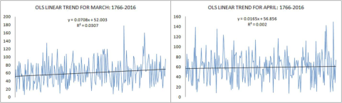
CHARTS 7-8: A COMPARISON OF THE 12 CALENDAR MONTHS

CHARTS 9-14: STANDARD DEVIATION IN A MOVING 30-YEAR WINDOW

CHARTS 15-20: EXTREME VALUES AND OUTLIERS