Archive for August 2020
THE ULTIMATE SOLUTION
Posted on: August 31, 2020
THIS POST OFFERS A SOLUTION TO ANTHROPOGENIC GLOBAL WARMING AND CLIMATE CHANGE THAT THREATENS MASS EXTINCTIONS AND THE END OF THE PLANET ITSELF AS DESCRIBED IN A RELATED POST: LINK https://tambonthongchai.com/2019/04/16/theend/
PART-1: THE RISE OF HUMANS ON EARTH AND THEIR COMPLETE CAPTURE OF THE PLANET


THE CLIMATE CHANGE DISASTER THUS CREATED


A GOD GIVEN SOLUTION ARRIVES IN THE FORM OF A PANDEMIC


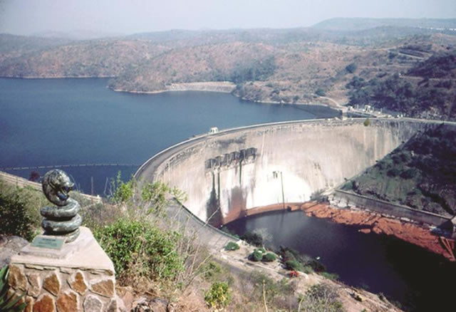
THE PLANET IS RETURNED TO ITS PRE-HUMAN PRISTINE CONDITION


- DISPLAYED ABOVE IS A VERTICAL SEQUENCE OF IMAGES THAT SHOW THE PRISTINE PLANET EARTH AS IT WAS BEFORE THE HUMANS TOOK OVER.
- THAT IS FOLLOWED BY A SEQUENCE OF THE ARRIVAL AND THE RISE OF HUMANS FROM HUNTER GATHERERS TO THE NEOLITHIC REVOLUTION AND FROM THERE TO THE INDUSTRIAL REVOLUTION AND POPULATION EXPLOSION THAT THREATENED THE END OF LIFE ON EARTH AND THE PLANET WITH CLIMATE CHANGE.
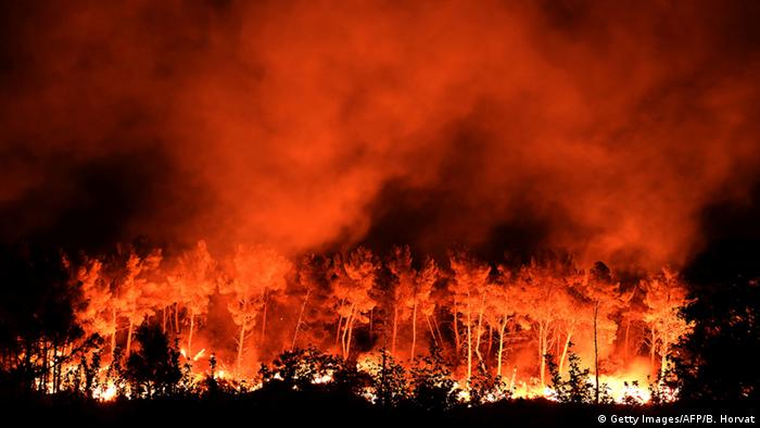
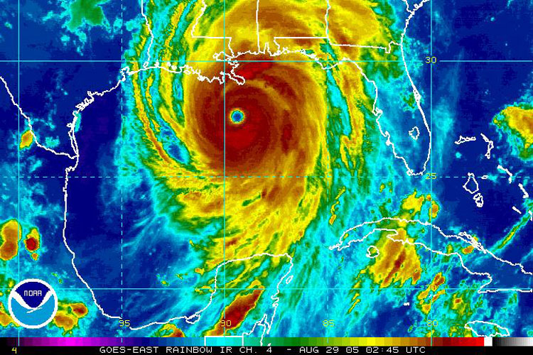
- THE CATASTROPHIC IMPACTS OF CLIMATE CHANGE ARE DISPLAYED IN THE IMAGES THAT FOLLOW.
- IT IS AT THAT POINT IN TIME THAT GOD INTERVENES AND SENDS THE COVID 19 PANDEMIC TO RID THE EARTH OF HUMANS AND THEREBY TO SAVE THE PLANET FROM CLIMATE CHANGE.
- THE IMAGES THAT FOLLOW SHOW HOW THE COVID 19 PANDEMIC COULD SAVE THE PLANET FROM HUMANS IN A GLOBAL VERSION OF JONESTOWN THAT WOULD TAKE OUT ALL HUMANS INCLUDING CLIMATE SCIENTISTS AND CLIMATE ACTIVISTS AND THE DEMOCRATCS BECAUSE THEY TOO ARE HUMAN BELIEVE IT OR NOT.
- THESE IMAGES SUGGEST THAT A CLEAR GOD GIVEN SOLUTION TO THE CLIMATE CRISIS IS THE COVID CRISIS.
- THE SOLUTION IS TO LET THE COVID PANDEMIC TAKE ITS COURSE AND THEREBY TO BRING ABOUT A GLOBAL VERSION OF JONESTOWN.
- THE GLOBAL JONESTOWN WILL BE BY WAY OF COVID NOT CYANIDE.
- IT WILL SAVE THE PLANET FROM CLIMATE CHANGE AND FROM HUMANS.
- https://youtu.be/OkookcrAnSE?list=TLPQMzEwODIwMjBGqMN2m5IkSw

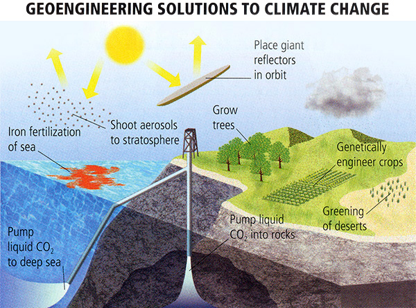
GEO-ENGINEERING CLIMATE CHANGE
Posted on: August 28, 2020
ABSTRACT: The most interesting aspect of the geoengineering debate is the difficult situation for climate science that it has created. Unlike climate deniers, geoengineering enthusiasts have fully bought into the climate science of fossil fuel emissions to global warming to catastrophic climate change. The fear based activism of climate science has worked well and these people are genuinely scared and genuinely concerned and wanting to help. In that sense they are close allies of climate change activists. Both sides believe in catastrophic climate change and both sides want to take climate action and the sooner the better. The only thing that separates them is their choice of climate action. And yet, just the difference in choice of climate action, sulfate aerosols on one side and the end of fossil fuels on the other, is enough to have created as much acrimony between these climate allies as there is between climate science activists and climate deniers.
The strong and uncompromising position of climate science is that there is no place and no role for geoengineering in their effort to save the planet from climate change. The only possible form of climate action acceptable in climate science is to bring about the end of fossil fuels. It is this issue and only this issue that has created the acrimony between climate science activism and geoengineering. The difficulty that climate science is having with their geoengineering climate action supporters serves therefore to bare the hidden agenda of climate science. This agenda holds that the only acceptable climate action to save the planet from climate change is the end of fossil fuels and that no alternative to that solution is acceptable.
This hard position of climate science implies that their real agenda is anti fossil fuel activism. This assessment explains the oddities of desperate climate science arguments against geoengineering as for example that geoengineering will reduce the efficiency of solar panels and photosynthesis that are needed to fight climate change although the geoengineering they are arguing against would make these arguments irrelevant. The concerted effort by climate science to create fear of geoengineering, calling it a “Pandora’s box” and instigator of war among nations serves as evidence of this difficult relationship as when someone falls in love with you for all the wrong reasons.
The complex and difficult relationship between climate science and geoengineering becomes clear when climate change activism is seen as anti-fossil fuel activism. The key to understanding the real underlying movement in climate science is that only the transition from fossil fuels to renewable energy is an acceptable solution.
RELATED POST ON THIS ISSUE: LINK https://tambonthongchai.com/2020/03/23/anti-fossil-fuel-activism-disguised-as-climate-science/

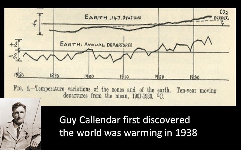
FIGURE 1: ETCW AND 1970S COOLING ANOMALIES

EARLY 20TH CENTURY WARMING AND THE 1970S COOLING ANOMALY
Global warming from 1930 to 1938, was identified in Callendar 1938, the world’s first AGW research paper, as “artificial global warming attributed to the fossil fuel emissions of the industrial economy
LINK https://tambonthongchai.com/2018/06/29/peer-review-comments-on-callendar-1938/
However, that warming ended soon after the publication of the Callendar 1938 paper as the world entered a 30-year cooling period 1945-1975 now known as the 1970s cooling anomaly
LINK https://tambonthongchai.com/2018/10/23/the-1970s-cooling-anomaly-of-agw/
As a result of the 1970s cooling, the warming identified by Guy Stewart Callendar as an artificial creation of the industrial economy is today understood very differently by climate science as a puzzling AGW anomaly referred to as the ETCW {Early Twentieth Century Warming} puzzle in AGW theory
LINK#1 https://tambonthongchai.com/2020/01/28/tcw/
LINK#2 https://tambonthongchai.com/2019/06/02/hegerl2018/
THE 1970S COOLING ANOMALY EXPLAINED BY STEPHEN SCHNEIDER

In the context of AGW climate change where fossil fuel emissions of the industrial economy cause warming, the 1945-1975 cooling anomaly took on a greater mystery because this period coincides with rapid postwar industrial growth and an explosive growth in automobile ownership.
The resolution of this mystery by the Late Great Stephen Schneider is now generally accepted as the explanation of the 1970s cooling anomaly in the context of AGW climate change. The genius of the Schneider CO2/Aerosol model of the impact of fossil fuel emissions on surface temperature is that it explains both warming and cooling in terms of fossil fuel emissions.
The warming part is the standard AGW theory that atmospheric CO2 concentration is linearly responsive to fossil fuel emissions and that surface temperature is logarithmically responsive to atmospheric CO2 concentration. The cooling part is that that emissions from fossil fuel combustion contain not only gaseous CO2 but also aerosols and sulfur dioxide (SO2) that when combined with water turns into acidic sulfate aerosol in what has been termed the “acid rain” issue in the EPA’s clean air act. Details of the acid rain issue are provided in a related post on acid rain LINK https://tambonthongchai.com/2019/03/12/acidrain/
The relevance of acid rain in the Schneider aerosol paper is that in general, sulfate aerosols are carried to the stratosphere where they reflect sunlight and cause cooling. The aerosol cooling effect is much stronger for sulfate aerosols. These were found in fossil fuel emissions prior to the EPA 1971 rule and the acid rain program against SO2 emissions.
An additional factor is that the warming effect of fossil fuel emissions in terms of atmospheric CO2 concentration is logarithmic whereas the cooling effect of aerosols goes up linearly with atmospheric concentration with the effect amplified by the aerosols that are already in the stratosphere.
These dynamics imply that the more CO2 there is in the atmosphere the lower the incremental warming effect of an incremental amount of CO2; BUT the more aerosol there is in the atmosphere the greater the incremental cooling effect effect of an incremental amount of aerosol. This means that when both CO2 and aerosols are going up at the same rate during a time of global warming, aerosol cooling will eventually overtake CO2 warming and the overall effect of fossil fuel emissions will be cooling particularly so in the presence of sulfate aerosols.
The Schneider theory of the 1970s cooling is that this is what had happened and why the 1970s cooling had occurred. Here is his story. The explosive growth in the use of fossil fuels without an EPA and without emission restrictions caused sulfate aerosol cooling to overcome CO2 GHG warming over the period roughly 1945 to 1975 as seen in these charts derived from the HadCRU global mean temperature reconstruction. And when SO2 emission restrictions were imposed in 1971, sulfate aerosol emissions began to fall until CO2 warming once again dominated.
The two GIF charts below trace the Schneider 1970s cooling period for the twelve calendar months one calendar month at a time cycling from January to December and back to January. The chart on the left plots the global mean surface temperature in red and its third order polynomial regression curve in black from 1930 to 1988. The chart on the right plots the decadal temperature trend for the decade ending in 1939 to the decade ending in 1988. The decadal window moves through the time series one year at a time. The blue line in the chart on the right is the zero trend marker. points above the blue line represent decadal warming and those below the blue line represent decadal cooling. What we see in these charts is that although there are significant differences among the calendar months, in most months, notably April to October, we do find the Schneider cooling somewhere in the 1945 yo 1975 region. These curves also reveal the ETCW
1988 was a significant year in the history of the AGW movement because it marks the Hansen Congressional Testimony LINK https://tambonthongchai.com/2019/05/09/hansen88/ that at once launched AGW fear based activism and led to the role of the UN as a global environmental agency fresh from its apparent ozone success at the Montreal Protocol with the flawed and failed assumption that it could repeat its Montreal Protocol ozone success in the Kyoto Protocol climate plan. Most importantly, it was also a time when global warming had fully recovered from its 1970s cooling anomaly.
Also of note in this regard is that because of the AGW confusion created by the backwards data of the 1970s cooling following the ETCW warming, many climate scientists find solace in the real clear AGW data from the end of the 1970s cooling even at the expense of the confirmation bias and circular reasoning that it implies. to the present as described in a related post LINK https://tambonthongchai.com/2018/08/24/climate-scientist-proves-human-cause/
However, the most intriguing outcome of the 1970s cooling and its explanation by Stephen Schneider is that: Since sulfate aerosols could reverse the strong and mysterious ETCW warming into the strong and mysterious 1970s cooling, then a similar aerosol human intervention serves as an alternative climate action plan to the costly and possibly unrealistic proposal of changing the energy infrastructure from fossil fuels to a renewables technology that is still a work in progress and not ready for large scale implementation without a fossil fueled backup LINK https://tambonthongchai.com/2020/08/18/energy-storage/ . The engineering design of many such aerosol intervention plans have been proposed in a field of research described as GEO-ENGINEERING by most and as CLIMATE REPAIR by Sir David King, a key deal maker in the Paris Agreement who now concedes that it has failed and that therefore CLIMATE REPAIR is the only remaining option.
A geo-engineering bibliography is provided below along with a well-written summary of the geo-engineering issue Published at the Yale School of the Environment LINK https://e360.yale.edu/features/geoengineer-the-planet-more-scientists-now-say-it-must-be-an-option
GEO-ENGINEERING ADVOCATES
MARCIA MCNUTT

DAVID KEITH
:no_upscale()/cdn.vox-cdn.com/uploads/chorus_asset/file/6455465/20140715_david_keith_portrait_uc_research_park_0104.0.jpg)
SIR DAVID KING

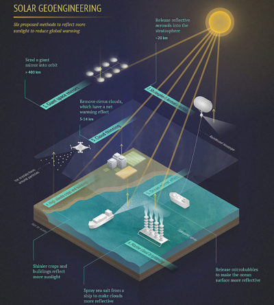
SOLAR GEO ENGINEERING OPTIONS (SOURCE YALE SCHOOL OF THE ENVIRONMENT)
SUMMARY OF THE YALE ASSESSMENT OF GEO-ENGINEERING
Once seen as spooky sci-fi, geoengineering is now being looked at with growing urgency . The failure of global emission reduction programs means we must consider controversial geoengineering technologies because we are running out of time. A geo-engineering research center has been established at Cambridge University. Technological options being considered are injecting sulfate aerosols into the stratosphere. In the USA the National Academies is studying sunlight reflection technologies. David Keith, a Harvard University physicist has developed technology for using chemistry to remove CO2 directly from the atmosphere. Kelly Wanser of the MARINE CLOUD BRIGHTENING Project is studying the efficacy of marine clouds (clouds above oceans) with SALTY OCEAN WATER to reflect more sunlight. As shown in the diagram below, this geoengineering technology increases the reflectiveness of clouds and is theoretically able to reduce global warming by 20%. Unlike aerosol sprays into the stratosphere, this form of geoengineering is controllable because it is a continuous process and can be moderated by ceasing the salt water sprays. A factor not usually taken into account and explained by PD Jones of the CRU is that cloud reflectiveness works both ways and it serves to warm the night by trapping terrestrial radiation as seen in the right frame of the diagram below.
China has an active government-funded geo-engineering research program. It has no plans for deployment, but is looking at how solar shading might slow the rapid melting of Himalayan glaciers.

Geoengineering the climate to halt global warming has been discussed almost as long as the threat of warming itself. American researchers in the 1960s suggested floating billions of white objects such as golf balls on the oceans to reflect sunlight. In 1977, Cesare Marchetti of Austria discussed ways of catching Europe’s CO2 emissions and injecting them into sinking Atlantic Ocean currents.
In 1982, Soviet scientist Mikhail Budyko proposed filling the stratosphere with sulphate particles to reflect sunlight back into space. Also fertilizing the oceans with iron stimulates growth of CO2-absorbing algae. Edward Teller, inventor of the hydrogen bomb, proposed putting giant mirrors into space.
Traditional climate scientists have regarded these proposals as heretical, because they undermine the case for urgent reductions in greenhouse gas emissions. A group of scientists writing in Nature as recently as April last year, called solar geoengineering “outlandish and unsettling… redolent of science fiction.”
But the mood is shifting because the window of opportunity to avoid breaching the Paris climate target of staying well below 2C is narrowing sharply. The rate of rise in CO2 emissions is increasing at a time when we should be making progress toward a goal of halving emissions by 2030. The CO2 concentrations in the atmosphere is the planet’s thermostat. It is now at 415 ppm and rising reaching levels not seen in 3 million years. We have two years left to bend the curve downward. We may be approaching a moment when nothing other than geoengineering will prevent “dangerous anthropogenic interference with the climate system. Myles Allen says that every year we are not reducing emissions is another 40 gigatons of CO2 in the atmosphere that we are committing future generations to remove.
Some downsides to geo-engineering have been identified. One researcher says that geo-engineering has a potential to promote conflict. According to Science Focus LINK https://www.sciencefocus.com/planet-earth/could-geoengineering-cause-a-climate-war/ one country’s geo-engineering could mess up the weather in another country and create political tension. that could lead to a climate war. Science Focus adds that there are other debilitating issues. For example, in geo-engineering technologies that remove CO2 from the atmosphere, there is no save place to store the CO2 to ensure permanent storage. And as for sulfate aerosol reflective technologies regional differences in the response would make it impossible to engineer a system that would work worldwide. Climate scientists point out that the climate system is too complex for such simplistic solutions. The impact of such geo-engineering systems is poorly understood and therefore artificial interference with this complex system could have unpredictable consequences. For example putting sulfate aerosols into the stratosphere could result in dangerous ozone depletion. We can’t take that chance.
A similar analysis by the Max Planck Institute LINK https://www.mpg.de/13374301/niemeier-climate-change-geoengineering finds that these well intended efforts to deal with global warming could backfire. Climate models show that the sulfate aerosol idea will indeed control the rise in temperature. It works in the climate models as long as we don’t also reduce fossil fuel emissions. The climate system could become unstable otherwise. Also, the models tell us that the sulfate aerosols will reduce precipitation and that could lead to devastating droughts. The climate system is too complex for such simplistic artificial interference.
The additional implication of this complexity and inability to predict or control the consequences could lead to war because the effects of national geoengineering programs cannot be limited to that nation state. Adverse effects felt in neighboring countries could lead to war.

SUMMARY AND CONCLUSION
:Geo-engineering seems an intrusive human meddling with nature with things like sulfate aerosol injection into the stratosphere that has no control knob and can’t be controlled or undone if unforeseen catastrophic effects such as cold weather, ozone depletion, or droughts evolve from this kind of meddling. It does not appear that these technologies have been properly thought through particularly so when one considers the absence of control. There is some solace in the sulfate aerosol technology as we have a well documented natural case record in the 1970s cooling but other than that, the technology needs to be proven and then developed to a high level or reliability and some ability to intervene and exercise needed control if things do go wrong. Prior to full scale implementation there should be test implementations to ensure function and safety. Lastly, there should be some way to undo the implementation if things don’t go as expected. As we have seen in the renewable energy fiasco described in a related post LINK https://tambonthongchai.com/2020/08/18/energy-storage/ rushing a technology to market before it is ready can end in disaster.
The more interesting aspect of the geoengineering debate is the difficult situation for climate science that it has created. Unlike climate deniers, geoengineering enthusiasts have fully bought into the climate science of fossil fuel emissions to global warming to catastrophic climate change. The fear based activism of climate science has worked well in these cases and these people are genuinely scared and genuinely concerned and wanting to help. In that sense they are close allies of climate change activists. Both sides believe in catastrophic climate change and both sides want to take climate action and the sooner the better. The only thing that separates them is their choice of climate action.
And yet, just the difference in choice of climate action – sulfate aerosols on one side and the end of fossil fuels on the other – is enough to have created as much distance between these groups as there is between climate science activists and climate deniers. For example, the climate science position is that there is no place and no role for geoengineering in their effort to save the planet from climate change. The only possible form of climate action acceptable to climate change activists is to bring about the end of fossil fuels. It is this distance between climate science activism and geoengineering activism that forces climate change activists to denigrate geoengineering and to create far fetched arguments against geoengineering such as the argument that geoengineering by country#1 might have an undesirable effect in neighboring country#2 that could lead to war between country#1 and country#2 although what geoengineering proponents propose is global climate action with global agreement just like climate scientists do. Also it is not possible to implement a country specific stratospheric sulfate aerosol program.
The difficulty that climate science activism is having with their geoengineering climate action partners serves therefore to bare the hidden agenda of climate science. This agenda implies that the only acceptable climate action to save the planet from climate change is the end of fossil fuels. That in turn serves as evidence that the real agenda of climate is anti fossil fuel activism LINK https://tambonthongchai.com/2020/03/23/anti-fossil-fuel-activism-disguised-as-climate-science/ LINK https://tambonthongchai.com/2020/08/18/energy-storage/
Climate science activism finds itself in the difficult situation of having been successful in creating fear of climate change but without the activism against fossil fuels that they had assumed would be the case. These difficulties are the source of the odd responses of climate science as for example that sulfate aerosols in the stratosphere will retard photosynthesis activity and even that aerosols will interfere with the solar energy scheme of climate science although the geoengineering they are arguing against would make solar power irrelevant.
The bibliography below sheds more light on the difficult task in climate science of having succeeded in scaring people with climate change without anticipating that a solution inconsistent with their anti fossil fuel activism may be proposed.
The concerted effort by climate science activists to create fear of geoengineering because it is the “Pandora’s box” shown below is strong evidence of this difficult relationship as when someone falls in love with you for all the wrong reasons. The complex and difficult disagreement between climate science activists and geoengineering activists is best understood in this context.

CLIMATE SCIENTIST: THE CASE AGAINST GEO-ENGINEERING
THE RELEVANT BIBLIOGRAPHY
- Schneider, Stephen H. “Geoengineering: could we or should we make it work?.” Philosophical Transactions of the Royal Society A: Mathematical, Physical and Engineering Sciences 366.1882 (2008): 3843-3862. Schemes to modify large-scale environment systems or control climate have been proposed for over 50 years to (i) increase temperatures in high latitudes, (ii) increase precipitation, (iii) decrease sea ice, (iv) create irrigation opportunities, or (v) offset potential global warming by injecting iron in the oceans or sea-salt aerosol in the marine boundary layer or spreading dust in the stratosphere to reflect away an amount of solar energy equivalent to the amount of heat trapped by increased greenhouse gases from human activities. These and other proposed geoengineering schemes are briefly reviewed. Recent schemes to intentionally modify climate have been proposed as either cheaper methods to counteract inadvertent climatic modifications than conventional mitigation techniques such as carbon taxes or pollutant emissions regulations or as a counter to rising emissions as governments delay policy action. Whereas proponents argue cost-effectiveness or the need to be prepared if mitigation and adaptation policies are not strong enough or enacted quickly enough to avoid the worst widespread impacts, critics point to the uncertainty that (i) any geoengineering scheme would work as planned or (ii) that the many centuries of international political stability and cooperation needed for the continuous maintenance of such schemes to offset century-long inadvertent effects is socially feasible. Moreover, the potential exists for transboundary conflicts should negative climatic events occur during geoengineering activities.
- Victor, David G. “On the regulation of geoengineering.” Oxford Review of Economic Policy 24.2 (2008): 322-336. New evidence that the climate system may be especially sensitive to the build-up of greenhouse gases and that humans are doing a poor job of controlling their effluent has animated discussions around the possibility of offsetting the human impact on climate through ‘geoengineering’. Nearly all assessments of geoengineering have concluded that the option, while ridden with flaws and unknown side effects, is intriguing because of its low cost and the ability for one or a few nations to geoengineer the planet without cooperation from others. I argue that norms to govern deployment of geoengineering systems will be needed soon. The standard instruments for establishing such norms, such as treaties, are unlikely to be effective in constraining geoengineers because the interests of key players diverge and it is relatively easy for countries to avoid inconvenient international commitments and act unilaterally. Instead, efforts to craft new norms ‘bottom up’ will be more effective. Such an approach, which would change the underlying interests of key countries and thus make them more willing to adopt binding norms in the future, will require active, open research programmes and assessments of geoengineering. Meaningful research may also require actual trial deployment of geoengineering systems so that norms are informed by relevant experience and command respect through use. Standard methods for international assessment organized by the Intergovernmental Panel on Climate Change (IPCC) are unlikely to yield useful evaluations of geoengineering options because the most important areas for assessment lie in the improbable, harmful, and unexpected side effects of geoengineering, not the ‘consensus science’ that IPCC does well. I also suggest that real-world geoengineering will be a lot more complex and expensive than currently thought because simple interventions—such as putting reflective particles in the stratosphere—will be combined with many other costlier interventions to offset nasty side effects.
- Ricke, Katharine, et al. “Unilateral geoengineering.” briefing notes for a workshop at the Council on Foreign Relations. Vol. 5. 2008. There are a variety of strategies, such as injecting light-reflecting particles into the stratosphere, that might be used to modify the Earth’s atmosphere-ocean system in an attempt to slow or reverse global warming. All of these “geoengineering” strategies involve great uncertainty and carry significant risks. They may not work as expected, imposing large unintended consequences on the climate system. While offsetting warming, most strategies are likely to leave other impacts unchecked, such as acidification of the ocean, the destruction of coral reefs, and changes in composition of terrestrial ecosystems. Yet, despite uncertain and very negative potential consequences, geoengineering might be needed to avert or reverse some dramatic change in the climate system, such as several meters of sea level rise that could impose disaster on hundreds of millions of people. Unlike the control of greenhouse gas emissions, which must be undertaken by all major emitting nations to be effective and is likely to be costly, geoengineering could be undertaken quickly and unilaterally by a single party, at relatively low cost. Unilateral geoengineering, however, is highly likely to impose costs on other countries and run risks with the entire planet’s climate system. This workshop will focus on the question of strategies for constraining and shaping geoengineering. We will explore formal, legal strategies as well as informal efforts to create norms that could govern testing and deployment of geoengineering systems and their possible undesirable consequences. We will probe whether it is possible to limit the use of geoengineering to circumstances of collective action by the international community in the face of true global emergencies and what might happen when there are disputes over when the emergency “trigger” should be pulled.
- Robock, Alan, et al. “Benefits, risks, and costs of stratospheric geoengineering.” Geophysical Research Letters 36.19 (2009). Injecting sulfate aerosol precursors into the stratosphere has been suggested as a means of geoengineering to cool the planet and reduce global warming. The decision to implement such a scheme would require a comparison of its benefits, dangers, and costs to those of other responses to global warming, including doing nothing. Here we evaluate those factors for stratospheric geoengineering with sulfate aerosols. Using existing U.S. military fighter and tanker planes, the annual costs of injecting aerosol precursors into the lower stratosphere would be several billion dollars. Using artillery or balloons to loft the gas would be much more expensive. We do not have enough information to evaluate more exotic techniques, such as pumping the gas up through a hose attached to a tower or balloon system. Anthropogenic stratospheric aerosol injection would cool the planet, stop the melting of sea ice and land‐based glaciers, slow sea level rise, and increase the terrestrial carbon sink, but produce regional drought, ozone depletion, less sunlight for solar power, and make skies less blue. Furthermore it would hamper Earth‐based optical astronomy, do nothing to stop ocean acidification, and present many ethical and moral issues. Further work is needed to quantify many of these factors to allow informed decision‐making.
- Jean Buck, Holly. “Geoengineering: Re‐making climate for profit or humanitarian intervention?.” Development and Change 43.1 (2012): 253-270. Climate engineering, or geoengineering, refers to large‐scale climate interventions to lower the earth’s temperature, either by blocking incoming sunlight or removing carbon dioxide from the biosphere. Regarded as ‘technofixes’ by critics, these strategies have evoked concern that they would extend the shelf life of fossil‐fuel driven socio‐ecological systems for far longer than they otherwise would, or should, endure. A critical reading views geoengineering as a class project that is designed to keep the climate system stable enough for existing production systems to continue operating. This article first examines these concerns, and then goes on to envision a regime driven by humanitarian agendas and concern for vulnerable populations, implemented through international development and aid institutions. The motivations of those who fund research and implement geoengineering techniques are important, as the rationale for developing geoengineering strategies will determine which techniques are pursued, and hence which ecologies are produced. The logic that shapes the geoengineering research process could potentially influence social ecologies centuries from now.
- Russell, Lynn M., et al. “Ecosystem impacts of geoengineering: a review for developing a science plan.” Ambio 41.4 (2012): 350-369. Geoengineering methods are intended to reduce climate change, which is already having demonstrable effects on ecosystem structure and functioning in some regions. Two types of geoengineering activities that have been proposed are: carbon dioxide (CO2) removal (CDR), which removes CO2 from the atmosphere, and solar radiation management (SRM, or sunlight reflection methods), which reflects a small percentage of sunlight back into space to offset warming from greenhouse gases (GHGs). Current research suggests that SRM or CDR might diminish the impacts of climate change on ecosystems by reducing changes in temperature and precipitation. However, sudden cessation of SRM would exacerbate the climate effects on ecosystems, and some CDR might interfere with oceanic and terrestrial ecosystem processes. The many risks and uncertainties associated with these new kinds of purposeful perturbations to the Earth system are not well understood and require cautious and comprehensive research.
- Vaughan, Naomi E., and Timothy M. Lenton. “A review of climate geoengineering proposals.” Climatic change 109.3-4 (2011): 745-790. Climate geoengineering proposals seek to rectify the current radiative imbalance via either (1) reducing incoming solar radiation (solar radiation management) or (2) removing CO2 from the atmosphere and transferring it to long-lived reservoirs (carbon dioxide removal). For each option, we discuss its effectiveness and potential side effects, also considering lifetime of effect, development and deployment timescale, reversibility, and failure risks. We present a detailed review that builds on earlier work by including the most recent literature, and is more extensive than previous comparative frameworks. Solar radiation management propsals are most effective but short-lived, whilst carbon dioxide removal measures gain effectiveness the longer they are pursued. Solar radiation management could restore the global radiative balance, but must be maintained to avoid abrupt warming, meanwhile ocean acidification and residual regional climate changes would still occur. Carbon dioxide removal involves less risk, and offers a way to return to a pre-industrial CO2 level and climate on a millennial timescale, but is potentially limited by the CO2 storage capacity of geological reservoirs. Geoengineering could complement mitigation, but it is not an alternative to it. We expand on the possible combinations of mitigation, carbon dioxide removal and solar radiation management that might be used to avoid dangerous climate change.

RELATED POST: THE END OF THE WORLD https://tambonthongchai.com/2019/04/16/theend/
Sir David Attenborough has said we need to ‘rewild the world’ by planting more forests and switch to a vegetarian diet in order to save the Earth. Speaking ahead of his new Netflix documentary film A Life On Our Planet, the 94-year-old naturalist warned it ‘cannot support millions of meat eaters‘. Calling on his decades of experience chronicling the natural world, he called for action to be taken immediately to save the global ‘pristine’ ecosystem that is ‘heading for disaster‘. The film, which will be released in the cinemas on September 28 before appearing on Netflix in the Autumn, will explore the defining moments of Sir David’s lifetime and the devastating changes he has witnessed. Sir David Attenborough has said we need to ‘rewild the planet’ and switch to a vegetarian diet in order to save the Earth. Speaking ahead of the launch, he said: ‘We must radically reduce the way we farm. We must change our diet. The planet can’t support billions of meat eaters. ‘If we had a mostly plant-based diet we could increase the yield of the land. We have an urgent need for free land. Forests are fundamental to recovery – bio-centres of diversity. ‘The wilder and more diverse the more effective. We must grow palm and soya on deforested lands. Nature is our biggest ally. ‘The living world is our unique marvel,’ he said. ‘The natural world is fading. This film is my vision of our future – our greatest mistake. ‘If we act now, we can put it right. This pristine of ecosystems is heading for disaster. Our imprint is global.
QUESTION: IF THIS ECOSYSTEM IS STILL PRISTINE AND THE PLANET IS STILL AROUND AND STILL ONLY HEADING FOR DISASTER 8,000 YEARS AFTER WE CAME OUT OF OUR CAVES IN THE FOREST TO START HUMAN CIVILIZATION IN THE NEOLITHIC REVOLUTION OF THE HOLOCENE CLIMATE OPTIMUM, WHY DO WE NEED TO GO BACK TO OUR CAVES IN THE FOREST TO SAVE THE PLANET?
RELATED POST: THE HOLOCENE CLIMATE OPTIMUM AND THE NEOLITHIC REVOLUTION https://tambonthongchai.com/2018/08/20/the-holocene-optimum-period-a-bibliography/
RELATED POST: THE COLLAPSE OF CIVILIZATION BY CLIMATE CHANGE https://tambonthongchai.com/2018/08/16/collapse/
RELATED POST: CLIMATE CHANGE AND THE END OF THE WORLD https://tambonthongchai.com/2019/04/16/theend/


AN EMOTIONAL FAREWELL TO THE NATURALIST WE USED TO LOVE OVER AT THE BUDBROMLEY BLOG https://budbromley.blog/author/budbromley/

CARBON BUDGET UNCERTAINTY
Posted on: August 26, 2020


THIS POST IS A CRITICAL REVIEW OF THE RESEARCH PAPER CITED BELOW. PICTURED ABOVE ARE WELL KNOWN CLIMATE SCIENTISTS RETO KNUTTI, JOERL ROGELJ, AND NATHAN GILLETT WHO ARE THREE OF THE EIGHT CO-AUTHORS OF THE PAPER BEING REVIEWED.
Uncertainty in carbon budget estimates due to internal climate variability
Katarzyna B Tokarska1, Vivek K Arora2, Nathan P Gillett2, Flavio Lehner1, Joeri Rogelj, Carl-Friedrich Schleussner4, Roland Séférian and Reto Knutti1, Accepted Manuscript online 13 August 2020 • © 2020 The Author(s). Published by IOP Publishing Ltd.
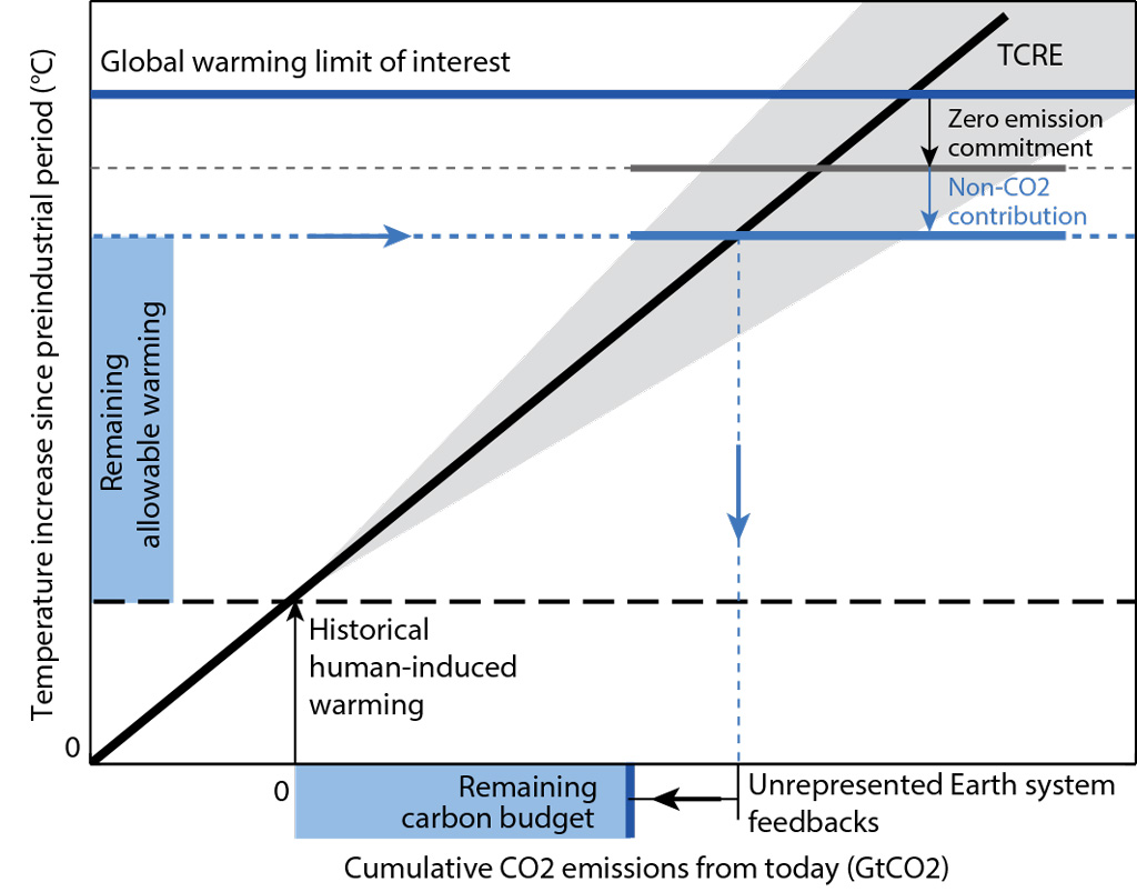
ABSTRACT: Remaining carbon budget specifies the cap on global cumulative CO2 emissions from the present-day onwards that would be in line with limiting global warming to a specific maximum level. In the context of the Paris Agreement, global warming is usually interpreted as the externally-forced response to anthropogenic activities and emissions, but it excludes the natural fluctuations of the climate system known as internal variability. A remaining carbon budget can be calculated from an estimate of the anthropogenic warming to date, and either (i) the ratio of CO2-induced warming to cumulative emissions, known as the Transient Climate Response to Emissions (TCRE), in addition to information on the temperature response to the future evolution of non-CO2 emissions; or (ii) climate model scenario simulations that reach a given temperature threshold. Here we quantify the impact of internal variability on the carbon budgets consistent with the Paris Agreement derived using either approach, and on the TCRE diagnosed from individual models. Our results show that internal variability contributes approximately ±0.09 °C to the overall uncertainty range of the human-induced warming to-date, leading to a spread in the remaining carbon budgets as large as ±50 PgC, when using approach (i). Differences in diagnosed TCRE due to internal variability in individual models can be as large as ±0.1 °C/1000 PgC (5-95% range). Alternatively, spread in the remaining carbon budgets calculated from (ii) using future concentration-driven simulations of large ensembles of CMIP6 and CMIP5 models is estimated at ± 30 PgC and ± 40 PgC (5-95% range). These results are important for model evaluation and imply that caution is needed when interpreting small remaining budgets in policy discussions. We do not question the validity of a carbon budget approach in determining mitigation requirements. However, due to intrinsic uncertainty arising from internal variability, it may only be possible to determine the exact year when a budget is exceeded in hindsight, highlighting the importance of a precautionary approach. FULL TEXT PDF: https://iopscience.iop.org/article/10.1088/1748-9326/abaf1b/pdf

RELATED POSTS
RELATED POST #7 DESCRIBES THE UNDERLYING STATISTICS ISSUE THAT CREATES THE TCRE FAUX CORRELATION. POST#8 DESCRIBES HOW THIS SPURIOUS CORRELATION CREATES FAUX CLIMATE SCIENCE ISSUES THAT HAVE NO RATIONAL INTERPRETATION OR SOLUTION AND LEADS CLIMATE SCIENCE TO ESM OF INCREASING COMPLEXITY SEEKING AN INTERPRETATION OF A SPURIOUS CORRELATION
- THE CARBON BUDGET CONUNDRUM https://tambonthongchai.com/2019/08/16/carbonbudgetconundrum/
- THE REMAINING CARBON BUDGET ANOMALY EXPLAINED https://tambonthongchai.com/?s=carbon+budget
- THE CARBON BUDGETS OF CLIMATE SCIENCE https://tambonthongchai.com/2019/09/21/boondoggle/
- CARBON BUDGETS AND THE TCRE https://tambonthongchai.com/2019/08/06/tcrebudget/
- ILLUSORY CARBON BUDGETS https://tambonthongchai.com/2019/08/02/illusorytcre/
- CARBON BUDGETS AND CLIMATE MITIGATION PATHWAYS https://tambonthongchai.com/2019/01/14/carbonbudget/
- TCRE: TRANSIENT CLIMATE RESPONSE TO CUMULATIVE EMISSIONS https://tambonthongchai.com/2018/05/06/tcre/
- STATISTICAL FLAWS CREATE CLIMATE SCIENCE CONFUSION https://tambonthongchai.com/2020/04/09/climate-statistics/


THE TCRE IS A SPURIOUS CORRELATION
THE TCRE CORRELATION DERIVES NOT FROM RESPONSIVENESS OF TEMPERATURE TO EMISSIONS BUT FROM A BIAS FOR POSITIVE VALUES IN THE TWO TIME SERIES AS FOLLOWS:
(1) EMISSIONS ARE ALWAYS POSITIVE, AND (2) DURING A TIME OF WARMING, ANNUAL CHANGES IN TEMPERATURE ARE MOSTLY POSITIVE.
IT IS THESE BIASES AND NOT A RESPONSIVENESS OF TEMPERATURE TO EMISSIONS THAT CREATES THE FAUX CORRELATION THAT HAS BEEN INTERPRETED AS A TEMPERATURE RESPONSE TO EMISSIONS DESCRIBED AS A “CLIMATE RESPONSE TO CUMULATIVE EMISSIONS” IN THE TCRE.
THE CREATION OF THE SPURIOUS TCRE CORRELATION IS DEMONSTRATED BELOW IN TWO GIF IMAGES.
EACH GIF IMAGE CYCLES THROUGH SEVEN RANDOM EMISSIONS AND TEMPERATURE DATA. IN THE FIRST GIF ANIMATION THERE ARE NO BIASES AND THE DATA ARE ACTUALLY RANDOM. THERE WE FIND NO CORRELATION AND A RANDOM TCRE OVER A WIDE RANGE OF VALUES BOTH POSITIVE AND NEGATIVE.
IN THE SECOND GIF ANIMATION, BIASES ARE INSERTED TO MIMIC THE ANNUAL EMISSIONS AND ANNUAL TEMPERATURE CHANGE DATA THAT ARE USED BY CLIMATE SCIENTISTS TO CONSTRUCT THE TCRE. THERE, ANNUAL EMISSIONS ARE ALWAYS POSITIVE AND DURING A TIME OF WARMING, THERE ARE MORE POSITIVE ANNUAL TEMPERATURE CHANGES THAN NEGATIVE. THERE WE FIND A STRONG CORRELATION AND THE TCRE METRIC THAT CLIMATE SCIENCE HAS MISTAKEN FOR A REAL CAUSE AND EFFECT PHENOMENON.
A FURTHER CONSIDERATION FOR THE SPURIOUSNESS OF THIS APPARENT CORRELATION RELATIONSHIP IS THAT A TIME SERIES OF THE CUMULATIVE VALUES OF ANOTHER TIME SERIES HAS NEITHER TIME SCALE NOR DEGREES OF FREEDOM. THIS TIME SERIES AND ITS CORRELATIONS HAVE NO INTERPRETATION IN TERMS OF THE EMISSIONS AND CLIMATE PHENOMENA THEY APPEAR TO REPRESENT.
THERE IS NO USEFUL INFORMATION IN THIS FAUX CORRELATION AND IT IS NOT POSSIBLE TO INTERPRET THIS CORRELATION AS EVIDENCE THAT EMISSIONS CAUSE WARMING OR AS A TOOL FOR CONSTRUCTING CLIMATE ACTION CARBON BUDGETS. THE REMAINING CARBON BUDGET ANOMALY IS A CREATION OF THIS FAUX CORRELATION AND NOT A REAL WORLD PHENOMENON THAT CAN BE UNDERSTOOD IN TERMS OF CLIMATE VARIABLES OR IN TERMS OF EARTH SYSTEM MODELS OF INCREASING LEVELS OF COMPLEXITY.
THE REMAINING CARBON BUDGET PUZZLE AND THE OTHER VEXING ISSUES IN THE TCRE CARBON BUDGET IS BEST UNDERSTOOD IN THESE TERMS AND NOT IN TERMS OF CLIMATE SCIENCE ISSUES THAT CAN BE SOLVED WITH CLIMATE SCIENCE OR EMS MODELS OF GREATER AND GREATER COMPLEXITY. THE PROBLEM IS A SPURIOUS CORRELATION. THE SOLUTION IS TO STOP INTERPRETING AND RELYING ON SPURIOUS CORRELATIONS TO UNDERSTAND HOW EMISSIONS CAUSE WARMING AND HOW TO TAKE CLIMATE ACTION TO MITIGATE THE RATE OF WARMING.
GIF IMAGE #1: NO BIAS FOR POSITIVE NUMBERS IN ANNUAL EMISSIONS OR IN ANNUAL TEMPERATURE CHANGE.

GIF IMAGE #2: WITH BIAS INSERTED. POSITIVE BIAS FOR ANNUAL TEMPERATURE CHANGE AND EMISSIONS ALWAYS POSITIVE.


TCRE CARBON BUDGET BIBLIOGRAPHY
- Matthews, H. Damon, et al. “The proportionality of global warming to cumulative carbon emissions.” Nature 459.7248 (2009): 829. The global temperature response to increasing atmospheric CO2 is often quantified by metrics such as equilibrium climate sensitivity and transient climate response1. These approaches, however, do not account for carbon cycle feedbacks and therefore do not fully represent the net response of the Earth system to anthropogenic CO2 emissions. Climate–carbon modelling experiments have shown that: (1) the warming per unit CO2 emitted does not depend on the background CO2 concentration2; (2) the total allowable emissions for climate stabilization do not depend on the timing of those emissions3,4,5; and (3) the temperature response to a pulse of CO2 is approximately constant on timescales of decades to centuries3,6,7,8. Here we generalize these results and show that the carbon–climate response (CCR), defined as the ratio of temperature change to cumulative carbon emissions, is approximately independent of both the atmospheric CO2 concentration and its rate of change on these timescales. From observational constraints, we estimate CCR to be in the range 1.0–2.1 °C per trillion tonnes of carbon (Tt C) emitted (5th to 95th percentiles), consistent with twenty-first-century CCR values simulated by climate–carbon models. Uncertainty in land-use CO2 emissions and aerosol forcing, however, means that higher observationally constrained values cannot be excluded. The CCR, when evaluated from climate–carbon models under idealized conditions, represents a simple yet robust metric for comparing models, which aggregates both climate feedbacks and carbon cycle feedbacks. CCR is also likely to be a useful concept for climate change mitigation and policy; by combining the uncertainties associated with climate sensitivity, carbon sinks and climate–carbon feedbacks into a single quantity, the CCR allows CO2-induced global mean temperature change to be inferred directly from cumulative carbon emissions.
- Allen, Myles R., et al. “Warming caused by cumulative carbon emissions towards the trillionth tonne.” Nature 458.7242 (2009): 1163. Global efforts to mitigate climate change are guided by projections of future temperatures1. But the eventual equilibrium global mean temperature associated with a given stabilization level of atmospheric greenhouse gas concentrations remains uncertain1,2,3, complicating the setting of stabilization targets to avoid potentially dangerous levels of global warming4,5,6,7,8. Similar problems apply to the carbon cycle: observations currently provide only a weak constraint on the response to future emissions9,10,11. Here we use ensemble simulations of simple climate-carbon-cycle models constrained by observations and projections from more comprehensive models to simulate the temperature response to a broad range of carbon dioxide emission pathways. We find that the peak warming caused by a given cumulative carbon dioxide emission is better constrained than the warming response to a stabilization scenario. Furthermore, the relationship between cumulative emissions and peak warming is remarkably insensitive to the emission pathway (timing of emissions or peak emission rate). Hence policy targets based on limiting cumulative emissions of carbon dioxide are likely to be more robust to scientific uncertainty than emission-rate or concentration targets. Total anthropogenic emissions of one trillion tonnes of carbon (3.67 trillion tonnes of CO2), about half of which has already been emitted since industrialization began, results in a most likely peak carbon-dioxide-induced warming of 2 °C above pre-industrial temperatures, with a 5–95% confidence interval of 1.3–3.9 °C.
- Mackey, Brendan, et al. “Untangling the confusion around land carbon science and climate change mitigation policy.” Nature climate change 3.6 (2013): 552. Depletion of ecosystem carbon stocks is a significant source of atmospheric CO2 and reducing land-based emissions and maintaining land carbon stocks contributes to climate change mitigation. We summarize current understanding about human perturbation of the global carbon cycle, examine three scientific issues and consider implications for the interpretation of international climate change policy decisions, concluding that considering carbon storage on land as a means to ‘offset’ CO2 emissions from burning fossil fuels (an idea with wide currency) is scientifically flawed. The capacity of terrestrial ecosystems to store carbon is finite and the current sequestration potential primarily reflects depletion due to past land use. Avoiding emissions from land carbon stocks and refilling depleted stocks reduces atmospheric CO2concentration, but the maximum amount of this reduction is equivalent to only a small fraction of potential fossil fuel emissions.
- Gignac, Renaud, and H. Damon Matthews. “Allocating a 2 C cumulative carbon budget to countries.” Environmental Research Letters 10.7 (2015): 075004. Recent estimates of the global carbon budget, or allowable cumulative CO2 emissions consistent with a given level of climate warming, have the potential to inform climate mitigation policy discussions aimed at maintaining global temperatures below 2 °C. This raises difficult questions, however, about how best to share this carbon budget amongst nations in a way that both respects the need for a finite cap on total allowable emissions, and also addresses the fundamental disparities amongst nations with respect to their historical and potential future emissions. Here we show how the contraction and convergence (C&C) framework can be applied to the division of a global carbon budget among nations, in a manner that both maintains total emissions below a level consistent with 2 °C, and also adheres to the principle of attaining equal per capita CO2emissions within the coming decades. We show further that historical differences in responsibility for climate warming can be quantified via a cumulative carbon debt (or credit), which represents the amount by which a given country’s historical emissions have exceeded (or fallen short of) the emissions that would have been consistent with their share of world population over time. This carbon debt/credit calculation enhances the potential utility of C&C, therefore providing a simple method to frame national climate mitigation targets in a way that both accounts for historical responsibility, and also respects the principle of international equity in determining future emissions allowances.
- Rogelj, Joeri, et al. “Mitigation choices impact carbon budget size compatible with low temperature goals.” Environmental Research Letters 10.7 (2015): 075003. Global-mean temperature increase is roughly proportional to cumulative emissions of carbon-dioxide (CO2). Limiting global warming to any level thus implies a finite CO2 budget. Due to geophysical uncertainties, the size of such budgets can only be expressed in probabilistic terms and is further influenced by non-CO2 emissions. We here explore how societal choices related to energy demand and specific mitigation options influence the size of carbon budgets for meeting a given temperature objective. We find that choices that exclude specific CO2mitigation technologies (like Carbon Capture and Storage) result in greater costs, smaller compatible CO2 budgets until 2050, but larger CO2 budgets until 2100. Vice versa, choices that lead to a larger CO2 mitigation potential result in CO2 budgets until 2100 that are smaller but can be met at lower costs. In most cases, these budget variations can be explained by the amount of non-CO2 mitigation that is carried out in conjunction with CO2, and associated global carbon prices that also drive mitigation of non-CO2 gases. Budget variations are of the order of 10% around their central value. In all cases, limiting warming to below 2 °C thus still implies that CO2 emissions need to be reduced rapidly in the coming decades.
- Riahi, Keywan, et al. “Locked into Copenhagen pledges—implications of short-term emission targets for the cost and feasibility of long-term climate goals.” Technological Forecasting and Social Change 90 (2015): 8-23. This paper provides an overview of the AMPERE modeling comparison project with focus on the implications of near-term policies for the costs and attainability of long-term climate objectives. Nine modeling teams participated in the project to explore the consequences of global emissions following the proposed policy stringency of the national pledges from the Copenhagen Accord and Cancún Agreements to 2030. Specific features compared to earlier assessments are the explicit consideration of near-term 2030 emission targets as well as the systematic sensitivity analysis for the availability and potential of mitigation technologies. Our estimates show that a 2030 mitigation effort comparable to the pledges would result in a further “lock-in” of the energy system into fossil fuels and thus impede the required energy transformation to reach low greenhouse-gas stabilization levels (450 ppm CO2e). Major implications include significant increases in mitigation costs, increased risk that low stabilization targets become unattainable, and reduced chances of staying below the proposed temperature change target of 2 °C in case of overshoot. With respect to technologies, we find that following the pledge pathways to 2030 would narrow policy choices, and increases the risks that some currently optional technologies, such as carbon capture and storage (CCS) or the large-scale deployment of bioenergy, will become “a must” by 2030.
- Rogelj, Joeri, et al. “Differences between carbon budget estimates unravelled.” Nature Climate Change 6.3 (2016): 245. Several methods exist to estimate the cumulative carbon emissions that would keep global warming to below a given temperature limit. Here we review estimates reported by the IPCC and the recent literature, and discuss the reasons underlying their differences. The most scientifically robust number — the carbon budget for CO2-induced warming only — is also the least relevant for real-world policy. Including all greenhouse gases and using methods based on scenarios that avoid instead of exceed a given temperature limit results in lower carbon budgets. For a >66% chance of limiting warming below the internationally agreed temperature limit of 2 °C relative to pre-industrial levels, the most appropriate carbon budget estimate is 590–1,240 GtCO2 from 2015 onwards. Variations within this range depend on the probability of staying below 2 °C and on end-of-century non-CO2 warming. Current CO2 emissions are about 40 GtCO2 yr−1, and global CO2 emissions thus have to be reduced urgently to keep within a 2 °C-compatible budget.
- Rogelj, Joeri, et al. “Paris Agreement climate proposals need a boost to keep warming well below 2 C.” Nature 534.7609 (2016): 631. The Paris climate agreement aims at holding global warming to well below 2 degrees Celsius and to “pursue efforts” to limit it to 1.5 degrees Celsius. To accomplish this, countries have submitted Intended Nationally Determined Contributions (INDCs) outlining their post-2020 climate action. Here we assess the effect of current INDCs on reducing aggregate greenhouse gas emissions, its implications for achieving the temperature objective of the Paris climate agreement, and potential options for overachievement. The INDCs collectively lower greenhouse gas emissions compared to where current policies stand, but still imply a median warming of 2.6–3.1 degrees Celsius by 2100. More can be achieved, because the agreement stipulates that targets for reducing greenhouse gas emissions are strengthened over time, both in ambition and scope. Substantial enhancement or over-delivery on current INDCs by additional national, sub-national and non-state actions is required to maintain a reasonable chance of meeting the target of keeping warming well below 2 degrees Celsius.
- Anderson, Kevin, and Glen Peters. “The trouble with negative emissions.” Science 354.6309 (2016): 182-183. In December 2015, member states of the United Nations Framework Convention on Climate Change (UNFCCC) adopted the Paris Agreement, which aims to hold the increase in the global average temperature to below 2°C and to pursue efforts to limit the temperature increase to 1.5°C. The Paris Agreement requires that anthropogenic greenhouse gas emission sources and sinks are balanced by the second half of this century. Because some nonzero sources are unavoidable, this leads to the abstract concept of “negative emissions,” the removal of carbon dioxide (CO2) from the atmosphere through technical means. The Integrated Assessment Models (IAMs) informing policy-makers assume the large-scale use of negative-emission technologies. If we rely on these and they are not deployed or are unsuccessful at removing CO2from the atmosphere at the levels assumed, society will be locked into a high-temperature pathway.
- Pfeiffer, Alexander, et al. “The ‘2 C capital stock’for electricity generation: Committed cumulative carbon emissions from the electricity generation sector and the transition to a green economy.” Applied Energy 179 (2016): 1395-1408. This paper defines the ‘2°C capital stock’ as the global stock of infrastructure which, if operated to the end of its normal economic life, implies global mean temperature increases of 2°C or more (with 50% probability). Using IPCC carbon budgets and the IPCC’s AR5 scenario database, and assuming future emissions from other sectors are compatible with a 2°C pathway, we calculate that the 2°C capital stock for electricity will be reached by 2017 based on current trends. In other words, even under the very optimistic assumption that other sectors reduce emissions in line with a 2°C target, no new emitting electricity infrastructure can be built after 2017 for this target to be met, unless other electricity infrastructure is retired early or retrofitted with carbon capture technologies. Policymakers and investors should question the economics of new long-lived energy infrastructure involving positive net emissions.
- Peters, Glen P., et al. “Key indicators to track current progress and future ambition of the Paris Agreement.” Nature Climate Change 7.2 (2017): 118. Current emission pledges to the Paris Agreement appear insufficient to hold the global average temperature increase to well below 2 °C above pre-industrial levels1. Yet, details are missing on how to track progress towards the ‘Paris goal’, inform the five-yearly ‘global stocktake’, and increase the ambition of Nationally Determined Contributions (NDCs). We develop a nested structure of key indicators to track progress through time. Global emissions2,3 track aggregated progress1, country-level decompositions track emerging trends4,5,6 that link directly to NDCs7, and technology diffusion8,9,10 indicates future reductions. We find the recent slowdown in global emissions growth11 is due to reduced growth in coal use since 2011, primarily in China and secondarily in the United States12. The slowdown is projected to continue in 2016, with global CO2 emissions from fossil fuels and industry similar to the 2015 level of 36 GtCO2. Explosive and policy-driven growth in wind and solar has contributed to the global emissions slowdown, but has been less important than economic factors and energy efficiency. We show that many key indicators are currently broadly consistent with emission scenarios that keep temperatures below 2 °C, but the continued lack of large-scale carbon capture and storage13 threatens 2030 targets and the longer-term Paris ambition of net-zero emissions.
- Millar, Richard J., et al. “Emission budgets and pathways consistent with limiting warming to 1.5 C.” Nature Geoscience10.10 (2017): 741. The Paris Agreement has opened debate on whether limiting warming to 1.5 °C is compatible with current emission pledges and warming of about 0.9 °C from the mid-nineteenth century to the present decade. We show that limiting cumulative post-2015 CO2 emissions to about 200 GtC would limit post-2015 warming to less than 0.6 °C in 66% of Earth system model members of the CMIP5 ensemble with no mitigation of other climate drivers. We combine a simple climate–carbon-cycle model with estimated ranges for key climate system properties from the IPCC Fifth Assessment Report. Assuming emissions peak and decline to below current levels by 2030, and continue thereafter on a much steeper decline, which would be historically unprecedented but consistent with a standard ambitious mitigation scenario (RCP2.6), results in a likely range of peak warming of 1.2–2.0 °C above the mid-nineteenth century. If CO2emissions are continuously adjusted over time to limit 2100 warming to 1.5 °C, with ambitious non-CO2 mitigation, net future cumulative CO2emissions are unlikely to prove less than 250 GtC and unlikely greater than 540 GtC. Hence, limiting warming to 1.5 °C is not yet a geophysical impossibility, but is likely to require delivery on strengthened pledges for 2030 followed by challengingly deep and rapid mitigation. Strengthening near-term emissions reductions would hedge against a high climate response or subsequent reduction rates proving economically, technically or politically unfeasible.
A MATHEMATICAL INCONSISTENCY
Posted on: August 26, 2020


THIS POST IS A COMPARISON OF THE ECS AND TCR, THE TWO METHODS USED INTERCHANGEABLY IN CLIMATE SCIENCE TO RELATE WARMING TO FOSSIL FUEL EMISSIONS. THE COMPARISON IS MADE IN TERMS OF MATHEMATICAL CONSISTENCY.
RELATED POST ON STATISTICS: LINK: https://tambonthongchai.com/2021/05/18/climate-science-vs-statistics/

THE EQUILIBRIUM CLIMATE SENSITIVITY ECS
The ECS measure of the impact of fossil fuel emissions on warming holds that atmospheric CO2 concentration at any given time is a linear function of cumulative emissions and that surface temperature is a logarithmic function of atmospheric CO2 concentration. These two relationships imply that surface temperature is a logarithmic function of cumulative emissions. That in turn implies that the amount of warming caused by a given level of cumulative emissions is the difference between the logarithms of the two cumulative emissions before and after.
TRANSIENT CLIMATE RESPONSE TO CUMULATIVE EMISSIONS TCR
The TCR measure of the impact of fossil fuel emissions on warming holds that the amount of warming is a linear function of cumulative emissions. This linearity is mathematically inconsistent with the ECS measure which implies that the amount of warming is proportional to the difference between the logarithms of the cumulative emissions before and after the period of warming under study.
IMPLICATIONS OF THIS MATHEMATICAL INCONSISTENCY
The mathematical inconsistency described above shows that the significant research effort in climate science to resolve the ECS and TCR measures of anthropogenic warming in terms of fossil fuel emissions with Earth System Models {ESM} is not possible because the two methods of computing the impact of emissions on temperature are not mathematically consistent and that makes it impossible for them to describe the same phenomenon in nature.
CONFIRMATION BIAS, CIRCULAR REASONING, AND MATHEMATICAL IMPOSSIBILITY OF EARTH SYSTEM MODELS {ESM}
In a related post on ESM {https://tambonthongchai.com/2020/08/25/earth-system-models-and-carbon-budgets/} we argue that the ESM construction procedure of beginning with the TCR warming derived from cumulative emissions and then explaining the result from an arbitrarily expanded list of ECS climate drivers is a form of circular reasoning. In this post we find that a further and more serious flaw in this procedure is the mathematical impossibility of the ESM exercise of reconciling ECS and TCR .
Yet another issue with the TCR and its Earth System Model application is that the TCR is based on a spurious correlation as shown in a related post: LINK: https://tambonthongchai.com/2019/04/30/illusory-statistical-power-in-time-series-analysis/
![PDF] Earth-system models of intermediate complexity | Semantic Scholar](https://d3i71xaburhd42.cloudfront.net/e25ec410d2783d2b3bec88fba2b49a6a51555c23/3-Figure2-1.png)
RELATED POST: WHAT THE TCRE TELLS US ABOUT CLIMATE SCIENCE
LINK: https://tambonthongchai.com/2021/11/18/tcre-transient-climate-response-to-cumulative-emissions/
THIS POST DESCRIBES THE USE OF EARTH SYSTEM MODELS (ESM) IN CLIMATE CHANGE RESEARCH AND EXPLORES THE LINK BETWEEN ESM AND TCR (TRANSIENT CLIMATE RESPONSE TO CUMULATIVE EMISSIONS)
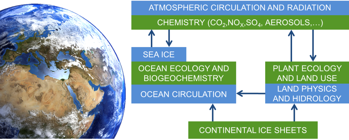
QUESTION: WHAT IS AN EARTH SYSTEM MODEL
ANSWER: A very readable paper on ESMs by IPCC Climate Scientist Dr. Gregory Flato is available online. Here is the link: http://citeseerx.ist.psu.edu/viewdoc/download?doi=10.1.1.662.1789&rep=rep1&type=pdf This post is a further exploration of his answer to this question.

PART-1: THE ESSENTIAL THEORY OF AGW AND ITS WEAKNESS
Historically, the original theory of anthropogenic global warming (AGW) and climate change proposed since Callendar 1938 and found in Revelle 1957, Charney 1979, Hansen 1981, Hansen 1988, IPCC 1990, IPCC 1996, IPCC 2001, IPCC 2007, Lacis 2010, IPCC 2014 and others has been consistently and uniformly stated as follows:
(1) Since the Industrial Revolution humans have been digging up and burning old carbon from under the ground and releasing carbon that is millions of years old into the atmosphere.
(2) This carbon is not a part of the current account of he carbon cycle and therefore an external perturbation of the carbon cycle with very old carbon and this perturbation changes atmospheric composition and causes atmospheric CO2 concentration to rise. This rise is therefore artificial and it is the human cause element of AGW theory.
(3) The rate of rise in atmospheric CO2 concentration seen in the data from Mauna Loa imply that about half of the fossil fuel emissions remain in the atmosphere, the so called “Airborne Fraction” while the other half becomes absorbed into carbon cycle sinks such as photosynthesis and ocean uptake.
(4) The surface temperature of the earth is a logarithmic function of the CO2 concentration of the atmosphere due to the heat trapping greenhouse effect of CO2. Therefore, as atmospheric CO2 rises, so does global mean surface temperature. This rise in temperature is therefore human caused by way of fossil fuel emissions. This is what makes global warming ANTHROPOGENIC and why we call it AGW.
(5) The empirical evidence of this causation sequence is that the theory predicts and the data show that temperature is a linear function of the natural logarithm of atmospheric CO2 concentration with a regression line slope that implies equilibrium climate sensitivity or ECS. The ECS relates the amount of warming for each doubling of atmospheric CO2 concentration.
(6) In 1979, Jule Charney consolidated results from five climate models to report Equilibrium Climate Sensitivity variously as ECS=[2.0-3.5], ECS=[2.6-4.1], and ECS=[1.5-4.5]. Charney then declared without elaborating that the most likely value of the ECS = 3 with its uncertainty indicated by the range ECS=[1.5-4.5] (Charney, 1979). This range was adopted by the IPCC and has since become dogma in climate science.
(7) However, there are unsettled and troublesome issues in this apparently empirically validated theory. The most well known issue, and one acknowledged by climate science, is UNCERTAINTY– that is the theory says that there is an ECS, and we can find the non-zero and non-negative ECS in the empirical evidence but we don’t know what the value of the ECS is exactly.
(8) This state of confusion in ECS research is best understood in terms of the following empirical results where some are purely observational while others are observational values constrained by climate models or climate model values constrained by observations : (Andronova, 2000) [2.0-5.0] ECS=[0.94-2.35]. (Gregory, 2002) [1.7 – 2.3], [1.4 – 7.7]. (Knutti, 2002) [2.7 – 8.7]. (Frame, 2005) [1.4–4.1], (Murphy, 2004) = [2.4–5.4] , (Stainforth, 2005) [1.9 – 11.5]. (Hegerl, 2006) [1.5-6.2]. (Kummer, 2017) [ 1.6-4.1]. Other estimates are ECS ≈ [1.2 – 7.7] for unconstrained observational [1.0 – 2.7], [1.0 – 3.5], [1.0 – 4.2], [1.3 – 4.9], [1.5 – 7.8], [1.5 – 7.3], and [1.0 – 7.0]. for observational ECS constrained by models. A more complete list is provided in a related post on this site https://tambonthongchai.com/2018/06/25/a-greenhouse-effect-of-atmospheric-co2/ .
(9) Climate science has responded to the uncertainty issue in various ways by using fudge factors such as the amount of ocean heat content change needed to smooth out and explain observational anomalies. Other climate science responses have included a biased interpretation of uncertainty by viewing uncertainty as a confidence interval and then altering the probability of the confidence interval placing a greater emphasis on the high end of the interval. Related post: https://tambonthongchai.com/2020/04/22/climate-science-uncertainty/
(10) In spite of these efforts, Uncertainty in the ECS grew into a contentious issue in climate science and nowhere more egregious than in the long range forecasts of future temperature by the IPCC that are used to motivate and construct climate action plans in terms reductions in fossil fuel emissions. The ECS uncertainty issue in climate science severely weakened the rationale for the principal policy implication of climate change research, that of reducing fossil fuel emissions to avoid catastrophic runaway warming by way of GHG forcing. This crisis in climate science created an urgent research agenda to resolve this core issue in the policy implications of climate change.
PART-2: TCRE: TRANSIENT CLIMATE RESPONSE TO CUMULATIVE EMISSIONS
(11): A breakthrough came in 2009 when three papers were published with an alternative to the failed ECS parameter that connects emissions to warming. All three of them proposed the same new causal connection between emissions and warming. These papers, the Matthews paper in particular, created a sensation in climate science as the community of scientists heaved a sigh of relief having re-established empirical evidence of human cause, crucial to the primary agenda of climate change research – that of reducing fossil fuel emissions and thereby moving the energy infrastructure away from fossil fuels. Here we present the paper by Damon Matthews.
(12) In 2009, Damon Matthews (and co-authors) submitted a paper to the journal Nature with an amazing discovery that could rescue climate science from the climate sensitivity uncertainty problem. He found a near perfect linear relationship and a near perfect correlation between cumulative fossil fuel emissions and surface temperature and proposed that the OLS linear regression coefficient of this line, expressed in Celsius units of warming per TTC (teratonnes of carbon equivalent) of cumulative emissions serves as an alternate measure of the global warming effect of emissions. This new and statistically stable rationale for attenuating warming by cutting fossil fuel emissions is thus proposed as a replacement for the failed ECS.
(13) The coefficient was named Transient Climate Response to Cumulative Emissions and was christened with the acronym TCRE and it quickly came to be accepted in climate science as a replacement for the failed ECS parameter.The TCRE became a sensational success. In accepting the (Matthews, 2009) paper for publication the editor of Nature wrote a congratulatory editorial comment as follows: “To date, efforts to describe and predict the climate response to human CO2 emissions have focused on climate sensitivity: the equilibrium temperature change associated with a doubling of CO2. But recent research has suggested that this ‘Charney’ sensitivity may be an incomplete representation of the full Earth system response, as it ignores changes in the carbon cycle, aerosols, land use and land cover. He continued: Matthews et al. propose a new measure, the transient climate response, or TCR. Using a combination of a simplified climate model, a range of simulations from a recent model inter-comparison, and historical constraints, they find that independent of the timing of emissions or the atmospheric concentration of CO2 emitting a trillion tonnes of carbon will cause 1.0 – 2.1 C of global warming, a TCRE value that is consistent with model predictions.
(14): The success of the TCRE as a foundational concept in relating climate change to emissions and thereby in developing carbon emission budgets for 2ºC and 1.5ºC warming targets led to its adoption by the IPCC in its AR5 report and also in its emergency call to the 1.5ºC carbon budget in the SR15 report of 2018. The initial value of 90%CI TCRE = [1.0 – 2.1]ºC per teratonne of cumulative emissions reported by Matthews was found to be very stable with later works reporting values within a narrow range of TCRE = [0.75-2.5] quite unlike the large range of ECS values listed in a related post [The Greenhouse Effect of Atmospheric CO2].
(15): The achievement was heralded by climate scientists around the world. A 2017 paper by converted ECS advocate Reto Knutti calls for discarding the ECS altogether and replacing it with the strong and stable TCRE as the primary climate science connection between emissions and warming. This connection is crucial to the anti fossil fuel activism function of AGW (Knutti 2017). In the Knutti 2017 paper titled “Beyond Equilibrium Climate Sensitivity”, he wrote “Estimates of the transient climate response are better constrained by observed warming and are more relevant for predicting warming over the next decades. Newer metrics relating global warming directly to the total emitted CO2 show that in order to keep warming to within 2 °C, future CO2 emissions have to remain strongly limited, irrespective of climate sensitivity being at the high or low end”.
(16): A crucial and attractive feature of the TCRE noted by Knutti and others is the relative ease and clarity with which the TCR can be translated into “carbon budgets” for any target amount of warming. A carbon budget is the amount of fossil fuel emissions that can be released to stay within a target amount of warming. For example, if TCR=2, then the carbon budget to keep warming within 2C is 1.0 teratonne and for a 1.5C target, the carbon budget is 0.75 teratonne, and so on. Thus, once the TCR was adopted by climate science as the new theory of human cause, climate action plans were presented in terms of carbon budgets constructed with the TCRE parameter.
(17): The success of the TCRE in terms of empirical verification and its practical application in the construction of carbon budgets notwithstanding, the construction of the TCRE contains a fatal statistical flaw that renders the TCRE a spurious statistic with no interpretation in terms of phenomena in the real world it apparently represents. These statistical issues are described in related posts: LINK#1: https://tambonthongchai.com/2018/05/06/tcre/ LINK#2: https://tambonthongchai.com/2018/12/03/tcruparody/
(18): The other issue is that the move from ECS to TCR created a vacuum in AGW theory. Whereas the ECS was based on the theory that atmospheric CO2 concentration is responsive to fossil fuel emissions and the theory that surface temperature is responsive to atmospheric CO2 concentration, the TCR is a purely empirical construct with no theoretical understanding of the climate science mechanism by which cumulative emissions drive surface temperature.
(19): The disconnect between climate change theory and the TCRE becomes apparent in terms of the mathematical inconsistencies described in a related post: LINK: https://tambonthongchai.com/2020/08/26/a-mathematical-inconsistency/ . The disconnection between theory and method creates confirmation bias in the use of the TCRE tool to rationalize observations in terms of flexible earth system models as described below. LINK to post on Confirmation Bias: https://tambonthongchai.com/2018/08/03/confirmationbias/
(20): This theoretical vacuum created a confirmation bias opportunity to explain any level of TCR warming in terms of any combination of a large number of known climate drivers and their positive and negative feedback mechanisms without the need for an exclusive focus on the GHG effect of atmospheric CO2 concentration in terms of a climate sensitivity parameter that had created the unresolved uncertainty issue in the original theory of AGW.
(21): Once the TCR warming forecast is accepted, climate science can then go through the data for all biogeochemical processes that can interact with the physical climate and their assumed interaction with the GHG effect of CO2 to explain the observed value of the TCR. These biogeochemical processes can include but are not limited to (1) carbon cycle flows, (2) the deep ocean beyond the “slab” surface layer concept, (3) the cooling effect of aerosols particularly sulfate aerosols, the various and poorly understood complex effect of clouds, and the impact of other anthropogenic chemicals in atmospheric composition such as ozone. These climate drivers, though not understood well enough to predict warming can nevertheless be interpreted in terms of the TCR warming in a confirmation bias logic that has become accepted procedure in climate science.
(22): The analysis begins with the TCR warming and then searches for known climate drivers that would explain the observed TCR. This unlimited extension of AGW theory is then incorporated into a new generation of climate models called ESM or Earth System Models. Unlike the older climate models that begin with emissions and predict warming with climate sensitivity, ESM analysis begins with emissions and the TCR warming and then searches for all possible explanations for the TCR warming in terms of known climate drivers. Although impressive in its expansive assessment of global warming, the procedure is a creation of confirmation bias and the statistical issues described in PART-3 below.
PART-3: STATISTICAL ISSUES IN THE TCR AND ESM. In the rush to the TCRE and to the carbon budgets constructed from the TCRE, and thereby to ESM climate models based on the TCRE as the starting point, climate science has overlooked some fundamental statistical issues. Surprisingly, these issues were ignored even after troublesome contradictions appeared in the use of the TCRE as the theory of AGW and the tool for the construction of carbon budgets in the climate action priority of AGW science.
One such issue apparently still unresolved in climate science is the remaining carbon budget. Briefly, the issue is that midway into a carbon budget period, the remaining carbon budget cannot be computed by subtraction. The unresolved struggle of climate science with the remaining carbon budget is highlighted in the bibliography below and also in related posts on this site where two of the papers listed in the bibliography are discussed. These are the Chris Jones and Pierre Friedlingstein 2020 paper https://tambonthongchai.com/2020/04/09/climate-statistics/ , and the Rogelj and Forster 2019 paper. https://tambonthongchai.com/2019/07/28/rcb/
What we find in these two papers is that the remaining carbon budget computed by subtraction of the emissions already made and that made with TCR computation for the remaining period do not match. This mismatch is then reconciled by the needed adjustments to the large suite of climate forcings and feedbacks in the ESM for the two time spans involved – a case of the same kind of confirmation bias and the Texas Sharpshooter fallacy that is used to construct the ESM explanation for the TCR . A detailed response to the Chris Jones and Pierre Friedlingstein 2020 paper points out the statistical flaws in the interpretation of the remaining carbon budget anomaly in terms of the ESM suite of convenience. LINK: https://tambonthongchai.com/2020/04/09/climate-statistics/ . An analysis of the remaining carbon budget issue is provided in a related post: LINK: https://tambonthongchai.com/2019/12/25/the-remaining-carbon-budget-anomaly-explained/
At the root of these complexities and the confused state of the ESM science of the TCR is that the TCR is based on a spurious correlation as explained in a related post LINK: https://tambonthongchai.com/2018/05/06/tcre/ .
As explained in the related post linked above, a time series of the cumulative values of another time series contains neither time scale nor degrees of freedom and therefore it does not contain useful information. The observed correlation derives from the sign pattern of the data in which emissions are always positive and in a period of warming, the annual warming is mostly positive. Under these conditions, the time series of cumulative values of annual emissions and annual warming will tend to be correlated although without time scale and without degrees of freedom. When the sign pattern is removed and randomized, the correlation vanishes.
The remaining carbon budget anomaly can be understood in this context. LINK: https://tambonthongchai.com/2019/12/25/the-remaining-carbon-budget-anomaly-explained/ . Since the annual warming that are positive is random, it is unlikely that the fraction of positive warming years in the two sub-periods will be the same.
Thus the only information content of strong correlations between cumulative values of time series data is that they happen to follow certain sign patterns. The further interpretation of these correlations and regression coefficients in terms of human cause of warming and in terms of carbon budgets is not possible. The attempt to interpret this correlation and its TCR regression coefficient in terms of climate change with the confirmation bias exercise of selecting ESM forcings to match the observed TCR does not yield useful information.
(23): A detailed response to the Chris Jones and Pierre Friedlingstein 2020 paper on TCRE carbon budgets provides further support for this conclusion. LINK: https://tambonthongchai.com/2020/04/09/climate-statistics/ . The summary of that review is reproduced below:
(24): ABSTRACT: Climate science has misinterpreted anomalies created by statistical errors as a climate science issue that needs to be resolved with climate models of greater complexity. In this context we find that their struggle with the remaining carbon budget puzzle demonstrates a failure of climate science to address statistical issues of the TCRE. This failure has led them down a complex and confusing path of trying to find a climate science explanation of the remaining carbon budget anomaly that was created by statistical errors. The research paper presented below serves as an example of this kind of climate research. The real solution to the remaining carbon budget puzzle is to understand the statistical flaws in the TCRE correlation described in the two linked documents and to stop using it [LINK] [LINK] . To drive home the point of the spuriousness of the TCRE correlation we show in the second linked document that the TCRE procedure that shows that fossil fuel emissions cause warming also shows that UFOs cause warming [LINK] .


RELATED POSTS ON TCRE CARBON BUDGETS
- ILLUSORY CARBON BUDGETS: https://tambonthongchai.com/2019/08/02/illusorytcre/
- CLIMATE SCIENCE VERSUS STATISTICS: https://tambonthongchai.com/2019/07/28/rcb/
- GRETA THUNBERG’S CARBON BUDGET: https://tambonthongchai.com/2020/01/02/greta-thunbergs-carbon-budget/
- THE REMAINING CARBON BUDGET EXPLAINED: https://tambonthongchai.com/2019/12/25/the-remaining-carbon-budget-anomaly-explained/
- THE REMAINING CARBON BUDGET ISSUE: https://tambonthongchai.com/2019/11/08/remainingcarbonbudget/
- THE TCR CARBON BUDGETS OF CLIMATE SCIENCE: https://tambonthongchai.com/?s=carbon+budget
- THE TCR CARBON BUDGET CONUNDRUM: https://tambonthongchai.com/2019/08/16/carbonbudgetconundrum/
- CARBON BUDGETS AND THE TCR: https://tambonthongchai.com/2019/08/06/tcrebudget/
- ILLUSORY CARBON BUDGETS: https://tambonthongchai.com/2019/08/02/illusorytcre/
- CARBON BUDGETS AND CLIMATE MITIGATION PATHWAYS: https://tambonthongchai.com/2019/01/14/carbonbudget/
(25): Yet another issue with the TCRE as a replacement of the ECS and the use of the TCRE to construct carbon budgets for a warming mechanism described in terms of the ECS is that the interpretation of ECS warming with the TCRE contains a fatal mathematical inconsistency as described in a related post: LINK: https://tambonthongchai.com/2020/08/26/a-mathematical-inconsistency/ . Briefly, “The ECS measure of the impact of fossil fuel emissions on warming holds that atmospheric CO2 concentration at any given time is a linear function of cumulative emissions and that surface temperature is a logarithmic function of atmospheric CO2 concentration. These two relationships imply that surface temperature is a logarithmic function of cumulative emissions. That in turn implies that the amount of warming caused by a given level of cumulative emissions is the difference between the logarithms of the two cumulative emissions before and after. The TCR measure of the impact of fossil fuel emissions on warming holds that the amount of warming is a linear function of cumulative emissions. This linearity is mathematically inconsistent with the ECS measure which implies that the amount of warming is proportional to the difference between the logarithms of the cumulative emissions before and after the period of warming under study. The mathematical inconsistency implies that the significant research effort in climate science to resolve the ECS and TCR measures of anthropogenic warming with Earth System Models {ESM} is not possible because the two methods of computing the impact of emissions on temperature are not mathematically consistent.
PART-4: THE RELEVANT BIBLIOGRAPHY
- The utility of the historical record for assessing the transient climate response to cumulative emissions
Richard J. Millar and Pierre Friedlingstein
Published:02 April 2018: https://doi.org/10.1098/rsta.2016.0449Abstract: The historical observational record offers a way to constrain the relationship between cumulative carbon dioxide emissions and global mean warming. We use a standard detection and attribution technique, along with observational uncertainties to estimate the all-forcing or ‘effective’ transient climate response to cumulative emissions (TCRE) from the observational record. Accounting for observational uncertainty and uncertainty in historical non-CO2 radiative forcing gives a best-estimate from the historical record of 1.84°C/TtC (1.43–2.37°C/TtC 5–95% uncertainty) for the effective TCRE and 1.31°C/TtC (0.88–2.60°C/TtC 5–95% uncertainty) for the CO2-only TCRE. While the best-estimate TCRE lies in the lower half of the IPCC likely range, the high upper bound is associated with the not-ruled-out possibility of a strongly negative aerosol forcing. Earth System Models have a higher effective TCRE range when compared like-for-like with the observations over the historical period, associated in part with a slight underestimate of diagnosed cumulative emissions relative to the observational best-estimate, a larger ensemble mean-simulated CO2-induced warming, and rapid post-2000 non-CO2 warming in some ensemble members. This article is part of the theme issue ‘The Paris Agreement: understanding the physical and social challenges for a warming world of 1.5°C above pre-industrial levels’. FULL TEXT https://royalsocietypublishing.org/doi/10.1098/rsta.2016.0449 - Jones, Chris D., and Pierre Friedlingstein. “Quantifying process-level uncertainty contributions to TCRE and Carbon Budgets for meeting Paris Agreement climate targets.” Environmental Research Letters (2020). To achieve the goals of the Paris Agreement requires deep and rapid reductions in anthropogenic CO2 emissions, but uncertainty surrounds the magnitude and depth of reductions. Earth system models provide a means to quantify the link from emissions to global climate change. Using the concept of TCRE—the transient climate response to cumulative carbon emissions—we can estimate the remaining carbon budget to achieve 1.5 or 2 °C. But the uncertainty is large, and this hinders the usefulness of the concept. Uncertainty in carbon budgets associated with a given global temperature rise is determined by the physical Earth system, and therefore Earth system modelling has a clear and high priority remit to address and reduce this uncertainty. Here we explore multi-model carbon cycle simulations across three generations of Earth system models to quantitatively assess the sources of uncertainty which propagate through to TCRE. Our analysis brings new insights which will allow us to determine how we can better direct our research priorities in order to reduce this uncertainty. We emphasise that uses of carbon budget estimates must bear in mind the uncertainty stemming from the biogeophysical Earth system, and we recommend specific areas where the carbon cycle research community needs to re-focus activity in order to try to reduce this uncertainty. We conclude that we should revise focus from the climate feedback on the carbon cycle to place more emphasis on CO2 as the main driver of carbon sinks and their long-term behaviour. Our proposed framework will enable multiple constraints on components of the carbon cycle to propagate to constraints on remaining carbon budgets. FULL TEXT: https://iopscience.iop.org/article/10.1088/1748-9326/ab858a/meta
- Ehlert, Dana, et al. “The sensitivity of the proportionality between temperature change and cumulative CO2 emissions to ocean mixing.” Journal of Climate 30.8 (2017): 2921-2935. The ratio of global mean surface air temperature change to cumulative CO2 emissions, referred to as transient climate response to cumulative CO2 emissions (TCRE), has been shown to be approximately constant on centennial time scales. The mechanisms behind this constancy are not well understood, but previous studies suggest that compensating effects of ocean heat and carbon fluxes, which are governed by the same ocean mixing processes, could be one cause for this approximate constancy. This hypothesis is investigated by forcing different versions of the University of Victoria Earth System Climate Model, which differ in the ocean mixing parameterization, with an idealized scenario of 1% annually increasing atmospheric CO2 until quadrupling of the preindustrial CO2 concentration and constant concentration thereafter. The relationship between surface air warming and cumulative emissions remains close to linear, but the TCRE varies between model versions, spanning the range of 1.2°–2.1°C EgC−1 at the time of CO2 doubling. For all model versions, the TCRE is not constant over time while atmospheric CO2 concentrations increase. It is constant after atmospheric CO2 stabilizes at 1120 ppm, because of compensating changes in temperature sensitivity (temperature change per unit radiative forcing) and cumulative airborne fraction. The TCRE remains approximately constant over time even if temperature sensitivity, determined by ocean heat flux, and cumulative airborne fraction, determined by ocean carbon flux, are taken from different model versions with different ocean mixing settings. This can partially be explained with temperature sensitivity and cumulative airborne fraction following similar trajectories, which suggests ocean heat and carbon fluxes scale approximately linearly with changes in vertical mixing. FULL TEXT: https://journals.ametsoc.org/jcli/article/30/8/2921/95100
- Rogelj, Joeri, et al. “Estimating and tracking the remaining carbon budget for stringent climate targets.” Nature 571.7765 (2019): 335-342. Research reported during the past decade has shown that global warming is roughly proportional to the total amount of carbon dioxide released into the atmosphere. This makes it possible to estimate the remaining carbon budget: the total amount of anthropogenic carbon dioxide that can still be emitted into the atmosphere while holding the global average temperature increase to the limit set by the Paris Agreement. However, a wide range of estimates for the remaining carbon budget has been reported, reducing the effectiveness of the remaining carbon budget as a means of setting emission reduction targets that are consistent with the Paris Agreement. Here we present a framework that enables us to track estimates of the remaining carbon budget and to understand how these estimates can improve over time as scientific knowledge advances. We propose that application of this framework may help to reconcile differences between estimates of the remaining carbon budget and may provide a basis for reducing uncertainty in the range of future estimates. FULL TEXT https://www.nature.com/articles/s41586-019-1368-z
- Tokarska, Katarzyna B., and Nathan P. Gillett. “Cumulative carbon emissions budgets consistent with 1.5 C global warming.” Nature Climate Change 8.4 (2018): 296-299. The Paris Agreement1 commits ratifying parties to pursue efforts to limit the global temperature increase to 1.5 °C relative to pre-industrial levels. Carbon budgets2,3,4,5 consistent with remaining below 1.5 °C warming, reported in the IPCC Fifth Assessment Report (AR5)2,6,8, are directly based on Earth system model (Coupled Model Intercomparison Project Phase 5)7 responses, which, on average, warm more than observations in response to historical CO2 emissions and other forcings8,9. These models indicate a median remaining budget of 55 PgC (ref. 10, base period: year 1870) left to emit from January 2016, the equivalent to approximately five years of emissions at the 2015 rate11,12. Here we calculate warming and carbon budgets relative to the decade 2006–2015, which eliminates model–observation differences in the climate–carbon response over the historical period9, and increases the median remaining carbon budget to 208 PgC (33–66% range of 130–255 PgC) from January 2016 (with mean warming of 0.89 °C for 2006–2015 relative to 1861–188013,14,15,16,17,18). There is little sensitivity to the observational data set used to infer warming that has occurred, and no significant dependence on the choice of emissions scenario. Thus, although limiting median projected global warming to below 1.5 °C is undoubtedly challenging19,20,21, our results indicate it is not impossible, as might be inferred from the IPCC AR5 carbon budgets.
- Mengis, Nadine, and H. Damon Matthews. “Non-CO 2 forcing changes will likely decrease the remaining carbon budget for 1.5° C.” npj Climate and Atmospheric Science 3.1 (2020): 1-7. One key contribution to the wide range of 1.5 °C carbon budgets among recent studies is the non-CO2 climate forcing scenario uncertainty. Based on a partitioning of historical non-CO2 forcing, we show that currently there is a net negative non-CO2 forcing from fossil fuel combustion (FFC), and a net positive non-CO2 climate forcing from land-use change (LUC) and agricultural activities. We perform a set of future simulations in which we prescribed a 1.5 °C temperature stabilisation trajectory, and diagnosed the resulting 1.5 °C carbon budgets. Using the historical partitioning, we then prescribed adjusted non-CO2 forcing scenarios consistent with our model’s simulated decrease in FFC CO2 emissions. We compared the diagnosed carbon budgets from these adjusted scenarios to those resulting from the default RCP scenario’s non-CO2 forcing, and to a scenario in which proportionality between future CO2 and non-CO2 forcing is assumed. We find a wide range of carbon budget estimates across scenarios, with the largest budget emerging from the scenario with assumed proportionality of CO2 and non-CO2 forcing. Furthermore, our adjusted-RCP scenarios produce carbon budgets that are smaller than the corresponding default RCP scenarios. Our results suggest that ambitious mitigation scenarios will likely be characterised by an increasing contribution of non-CO2 forcing, and that an assumption of continued proportionality between CO2 and non-CO2 forcing would lead to an overestimate of the remaining carbon budget. Maintaining such proportionality under ambitious fossil fuel mitigation would require mitigation of non-CO2 emissions at a rate that is substantially faster than found in the standard RCP scenarios. FULL TEXT https://www.nature.com/articles/s41612-020-0123-3
- Jones, Chris, et al. “Twenty-first-century compatible CO2 emissions and airborne fraction simulated by CMIP5 earth system models under four representative concentration pathways.” Journal of Climate 26.13 (2013): 4398-4413. The carbon cycle is a crucial Earth system component affecting climate and atmospheric composition. The response of natural carbon uptake to CO2 and climate change will determine anthropogenic emissions compatible with a target CO2 pathway. For phase 5 of the Coupled Model Intercomparison Project (CMIP5), four future representative concentration pathways (RCPs) have been generated by integrated assessment models (IAMs) and used as scenarios by state-of-the-art climate models, enabling quantification of compatible carbon emissions for the four scenarios by complex, process-based models. Here, the authors present results from 15 such Earth system GCMs for future changes in land and ocean carbon storage and the implications for anthropogenic emissions. The results are consistent with the underlying scenarios but show substantial model spread. Uncertainty in land carbon uptake due to differences among models is comparable with the spread across scenarios. Model estimates of historical fossil-fuel emissions agree well with reconstructions, and future projections for representative concentration pathway 2.6 (RCP2.6) and RCP4.5 are consistent with the IAMs. For high-end scenarios (RCP6.0 and RCP8.5), GCMs simulate smaller compatible emissions than the IAMs, indicating a larger climate–carbon cycle feedback in the GCMs in these scenarios. For the RCP2.6 mitigation scenario, an average reduction of 50% in emissions by 2050 from 1990 levels is required but with very large model spread (14%–96%). The models also disagree on both the requirement for sustained negative emissions to achieve the RCP2.6 CO2 concentration and the success of this scenario to restrict global warming below 2°C. All models agree that the future airborne fraction depends strongly on the emissions profile with higher airborne fraction for higher emissions scenarios. FULL TEXT https://journals.ametsoc.org/jcli/article/26/13/4398/34280
- Anav, A., et al. “Evaluating the land and ocean components of the global carbon cycle in the CMIP5 earth system models.” Journal of Climate 26.18 (2013): 6801-6843. The authors assess the ability of 18 Earth system models to simulate the land and ocean carbon cycle for the present climate. These models will be used in the next Intergovernmental Panel on Climate Change (IPCC) Fifth Assessment Report (AR5) for climate projections, and such evaluation allows identification of the strengths and weaknesses of individual coupled carbon–climate models as well as identification of systematic biases of the models. Results show that models correctly reproduce the main climatic variables controlling the spatial and temporal characteristics of the carbon cycle. The seasonal evolution of the variables under examination is well captured. However, weaknesses appear when reproducing specific fields: in particular, considering the land carbon cycle, a general overestimation of photosynthesis and leaf area index is found for most of the models, while the ocean evaluation shows that quite a few models underestimate the primary production.The authors also propose climate and carbon cycle performance metrics in order to assess whether there is a set of consistently better models for reproducing the carbon cycle. Averaged seasonal cycles and probability density functions (PDFs) calculated from model simulations are compared with the corresponding seasonal cycles and PDFs from different observed datasets. Although the metrics used in this study allow identification of some models as better or worse than the average, the ranking of this study is partially subjective because of the choice of the variables under examination and also can be sensitive to the choice of reference data. In addition, it was found that the model performances show significant regional variations. FULL TEXT https://journals.ametsoc.org/jcli/article/26/18/6801/34409
- Stevens, Bjorn, and Sandrine Bony. “What are climate models missing?.” Science 340.6136 (2013): 1053-1054. Fifty years ago, Joseph Smagorinsky published a landmark paper (1) describing numerical experiments using the primitive equations (a set of fluid equations that describe global atmospheric flows). In so doing, he introduced what later became known as a General Circulation Model (GCM). GCMs have come to provide a compelling framework for coupling the atmospheric circulation to a great variety of processes. Although early GCMs could only consider a small subset of these processes, it was widely appreciated that a more comprehensive treatment was necessary to adequately represent the drivers of the circulation. But how comprehensive this treatment must be was unclear and, as Smagorinsky realized (2), could only be determined through numerical experimentation. These types of experiments have since shown that an adequate description of basic processes like cloud formation, moist convection, and mixing is what climate models miss most. FULL TEXT https://science.sciencemag.org/content/340/6136/1053.full
- Anderson, Thomas R., Ed Hawkins, and Philip D. Jones. “CO2, the greenhouse effect and global warming: from the pioneering work of Arrhenius and Callendar to today’s Earth System Models.” Endeavour 40.3 (2016): 178-187. Climate warming during the course of the twenty-first century is projected to be between 1.0 and 3.7 °C depending on future greenhouse gas emissions, based on the ensemble-mean results of state-of-the-art Earth System Models (ESMs). Just how reliable are these projections, given the complexity of the climate system? The early history of climate research provides insight into the understanding and science needed to answer this question. We examine the mathematical quantifications of planetary energy budget developed by Svante Arrhenius (1859–1927) and Guy Stewart Callendar (1898–1964) and construct an empirical approximation of the latter, which we show to be successful at retrospectively predicting global warming over the course of the twentieth century. This approximation is then used to calculate warming in response to increasing atmospheric greenhouse gases during the twenty-first century, projecting a temperature increase at the lower bound of results generated by an ensemble of ESMs (as presented in the latest assessment by the Intergovernmental Panel on Climate Change). This result can be interpreted as follows. The climate system is conceptually complex but has at its heart the physical laws of radiative transfer. This basic, or “core” physics is relatively straightforward to compute mathematically, as exemplified by Callendar’s calculations, leading to quantitatively robust projections of baseline warming. The ESMs include not only the physical core but also climate feedbacks that introduce uncertainty into the projections in terms of magnitude, but not sign: positive (amplification of warming). As such, the projections of end-of-century global warming by ESMs are fundamentally trustworthy: quantitatively robust baseline warming based on the well-understood physics of radiative transfer, with extra warming due to climate feedbacks. These projections thus provide a compelling case that global climate will continue to undergo significant warming in response to ongoing emissions of CO2 and other greenhouse gases to the atmosphere. FULL TEXT https://www.sciencedirect.com/science/article/pii/S0160932716300308
- Bentsen, Mats, et al. “The Norwegian earth system model, NorESM1-M-Part 1: Description and basic evaluation.” GMDD 5.3 (2012): 2843-2931. The core version of the Norwegian Climate Center’s Earth System Model, named NorESM1-M, is presented. The NorESM-family of models are based on the Community Climate System Model version 4 (CCSM4) of the University Corporation for Atmospheric Research, but differs from the latter by, in particular, an isopycnic coordinate ocean model and advanced chemistry-aerosol-cloud-radiation interaction schemes. NorESM1-M has a horizontal resolution of approximately 2° for the atmosphere and land components and 1° for the ocean and ice components. NorESM is also available in a lower resolution version (NorESM1-L) and a version that includes prognostic biogeochemical cycling (NorESM1-ME). The latter two model configurations are not part of this paper. Here, a first-order assessment of the model stability, the mean model state and the internal variability based on the model experiments made available to CMIP5 are presented. Further analysis of the model performance is provided in an accompanying paper (Iversen et al., 2012), presenting the corresponding climate response and scenario projections made with NorESM1-M. FULL TEXT PDF https://gmd.copernicus.org/preprints/5/2843/2012/gmdd-5-2843-2012.pdf
- McMullin, Barry, et al. “Assessing negative carbon dioxide emissions from the perspective of a national “fair share” of the remaining global carbon budget.” Mitigation and Adaptation Strategies for Global Change (2019): 1-24. We present an assessment of the plausible Paris-aligned fair share net cumulative carbon dioxide (CO2) quota for an example nation state, the Republic of Ireland. By Paris-aligned, we mean consistent with the Paris Agreement adopted at the 21st Conference of the Parties to the United Nations Framework Convention on Climate Change, at Paris, France, in December 2015 (UNFCCC 2015). We compare and contrast this quota with both the aspirations expressed in the current Irish National Policy Position and current national emission projections. The fair share quota is assessed as a maximum of c. 391 million tonnes of carbon dioxide (MtCO2), equal to 83 tonnes of carbon dioxide (tCO2) per capita, from 2015, based on a precautionary estimate of the global carbon budget (GCB) and specific interpretation of global equity. Given Ireland’s high current CO2 per capita emission rate, this would correspond to sustained year-on-year reductions in nett annual CO2 emissions of over − 11% per year (beginning as of 2016). By contrast, the CO2 mitigation target indicated in the National Policy Position corresponds to nett annual reduction rates in the range of only −4.7% per year (low ambition) up to a maximum of − 8.3% per year (high ambition), and projections based on current and immediately planned mitigation measures indicate the possibility, instead, of sustained increases in emissions at a rate of the order of + 0.7% per year. Accordingly, there is a large gap between Paris-aligned ambition and current political and policy reality on the ground, with a significant risk of early emergence of “CO2 debt” and tacit reliance on rapid deployment of currently speculative (at a relevant scale and feasible cost) negative CO2 emission technologies to actively remove CO2 from the atmosphere. While the detailed policy situation will clearly differ from country to country, we suggest that this methodology, and its CO2debt framing, may be usefully applied in other individual countries or regions. We recommend that such framing be incorporated explicitly into a global mitigation strategy via the statements of nationally determined contributions required to be submitted and updated by all parties under the Paris Agreement processes.
- Flato, Gregory M. “Earth system models: an overview.” Wiley Interdisciplinary Reviews: Climate Change 2.6 (2011): 783-800. Earth System models (ESMs) are global climate models with the added capability to explicitly represent biogeochemical processes that interact with the physical climate and so alter its response to forcing such as that associated with human‐caused emissions of greenhouse gases. Representing the global carbon cycle allows for feedbacks between the physical climate and the biological and chemical processes in the ocean and on land that take up some of the emitted carbon dioxide and so act to reduce warming. The sulfur cycle is also important in that both natural and human emissions of sulfur contribute to the production of sulfate aerosols which reflect incoming solar radiation (a direct cooling effect) and alter cloud properties (an indirect cooling effect). Other components such as ozone are also being incorporated into some ESMs. Evaluating the physical component of an ESM is becoming increasingly comprehensive and sophisticated, but the evaluation of the biogeochemical components suffer somewhat from a lack of comprehensive global‐scale observational data. Nevertheless, such models provide valuable insight into climate variability and change, and the role of human activities and possible mitigation actions on future climate change. Internationally coordinated experiments are increasingly important in providing a multimodel ensemble of climate simulations, thereby taking advantage of some ‘cancellation of errors’ and allowing better quantification of uncertainty. WIREs Clim Change 2011, 2:783–800. doi: 10.1002/wcc.148 FULL TEXT PDF http://citeseerx.ist.psu.edu/viewdoc/download?doi=10.1.1.662.1789&rep=rep1&type=pdf
- McPhaden, Michael J., Stephen E. Zebiak, and Michael H. Glantz. “ENSO as an integrating concept in earth science.” science 314.5806 (2006): 1740-1745. The El Niño–Southern Oscillation (ENSO) cycle of alternating warm El Niño and cold La Niña events is the dominant year-to-year climate signal on Earth. ENSO originates in the tropical Pacific through interactions between the ocean and the atmosphere, but its environmental and socioeconomic impacts are felt worldwide. Spurred on by the powerful 1997–1998 El Niño, efforts to understand the causes and consequences of ENSO have greatly expanded in the past few years. These efforts reveal the breadth of ENSO’s influence on the Earth system and the potential to exploit its predictability for societal benefit. However, many intertwined issues regarding ENSO dynamics, impacts, forecasting, and applications remain unresolved. Research to address these issues will not only lead to progress across a broad range of scientific disciplines but also provide an opportunity to educate the public and policy makers about the importance of climate variability and change in the modern world. FULL TEXT https://science.sciencemag.org/content/314/5806/1740.full
- Clark, Martyn P., et al. “Improving the representation of hydrologic processes in Earth System Models.” Water Resources Research 51.8 (2015): 5929-5956. Many of the scientific and societal challenges in understanding and preparing for global environmental change rest upon our ability to understand and predict the water cycle change at large river basin, continent, and global scales. However, current large‐scale land models (as a component of Earth System Models, or ESMs) do not yet reflect the best hydrologic process understanding or utilize the large amount of hydrologic observations for model testing. This paper discusses the opportunities and key challenges to improve hydrologic process representations and benchmarking in ESM land models, suggesting that (1) land model development can benefit from recent advances in hydrology, both through incorporating key processes (e.g., groundwater‐surface water interactions) and new approaches to describe multiscale spatial variability and hydrologic connectivity; (2) accelerating model advances requires comprehensive hydrologic benchmarking in order to systematically evaluate competing alternatives, understand model weaknesses, and prioritize model development needs, and (3) stronger collaboration is needed between the hydrology and ESM modeling communities, both through greater engagement of hydrologists in ESM land model development, and through rigorous evaluation of ESM hydrology performance in research watersheds or Critical Zone Observatories. Such coordinated efforts in advancing hydrology in ESMs have the potential to substantially impact energy, carbon, and nutrient cycle prediction capabilities through the fundamental role hydrologic processes play in regulating these cycles. FULL TEXT https://agupubs.onlinelibrary.wiley.com/doi/full/10.1002/2015WR017096%4010.1002/%28ISSN%291944-7973.WRR50
- Fisher, Rosie A., et al. “Vegetation demographics in Earth System Models: A review of progress and priorities.” Global change biology 24.1 (2018): 35-54. Numerous current efforts seek to improve the representation of ecosystem ecology and vegetation demographic processes within Earth System Models (ESMs). These developments are widely viewed as an important step in developing greater realism in predictions of future ecosystem states and fluxes. Increased realism, however, leads to increased model complexity, with new features raising a suite of ecological questions that require empirical constraints. Here, we review the developments that permit the representation of plant demographics in ESMs, and identify issues raised by these developments that highlight important gaps in ecological understanding. These issues inevitably translate into uncertainty in model projections but also allow models to be applied to new processes and questions concerning the dynamics of real‐world ecosystems. We argue that stronger and more innovative connections to data, across the range of scales considered, are required to address these gaps in understanding. The development of first‐generation land surface models as a unifying framework for ecophysiological understanding stimulated much research into plant physiological traits and gas exchange. Constraining predictions at ecologically relevant spatial and temporal scales will require a similar investment of effort and intensified inter‐disciplinary communication. FULL TEXT PDF https://onlinelibrary.wiley.com/doi/epdf/10.1111/gcb.13910
- Getzlaff, Julia, and Heiner Dietze. “Effects of increased isopycnal diffusivity mimicking the unresolved equatorial intermediate current system in an earth system climate model.” Geophysical Research Letters 40.10 (2013): 2166-2170. Earth system climate models generally underestimate dissolved oxygen concentrations in the deep eastern equatorial Pacific. This problem is associated with the “nutrient trapping” problem, described by Najjar et al. [1992], and is, at least partially, caused by a deficient representation of the Equatorial Intermediate Current System (EICS). Here we emulate the unresolved EICS in the UVic earth system climate model by locally increasing the zonal isopycnal diffusivity. An anisotropic diffusivity of ∼50,000 m2 s−1 yields an improved global representation of temperature, salinity and oxygen. In addition, it (1) resolves most of the local “nutrient trapping” and associated oxygen deficit in the eastern equatorial Pacific and (2) reduces spurious zonal temperature gradients on isopycnals without affecting other physical metrics such as meridional overturning or air‐sea heat fluxes. Finally, climate projections of low‐oxygenated waters and associated denitrification change sign and apparently become more plausible. FULL TEXT https://agupubs.onlinelibrary.wiley.com/doi/full/10.1002/grl.50419
- Pielke Sr, Roger A., et al. “Unresolved issues with the assessment of multidecadal global land surface temperature trends.” Journal of Geophysical Research: Atmospheres 112.D24 (2007). This paper documents various unresolved issues in using surface temperature trends as a metric for assessing global and regional climate change. A series of examples ranging from errors caused by temperature measurements at a monitoring station to the undocumented biases in the regionally and globally averaged time series are provided. The issues are poorly understood or documented and relate to micrometeorological impacts due to warm bias in nighttime minimum temperatures, poor siting of the instrumentation, effect of winds as well as surface atmospheric water vapor content on temperature trends, the quantification of uncertainties in the homogenization of surface temperature data, and the influence of land use/land cover (LULC) change on surface temperature trends. Because of the issues presented in this paper related to the analysis of multidecadal surface temperature we recommend that greater, more complete documentation and quantification of these issues be required for all observation stations that are intended to be used in such assessments. This is necessary for confidence in the actual observations of surface temperature variability and long‐term trends. FULL TEXT https://agupubs.onlinelibrary.wiley.com/doi/full/10.1029/2006JD008229
MYSTERIES OF THE UPPER ATMOSPHERE
Posted on: August 23, 2020


THIS POST IS A CRITICAL REVIEW OF THE ARTICLE
ANTARCTIC RESEARCH UNLOCKS MYSTERIES OF THE UPPER ATMOSPHERE, Home News and media 2020 Antarctic research unlocks mysteries of the upper atmosphere 27 JULY 2020
A long-term study in Antarctica of the upper atmosphere in the coldest place on Earth reveals several new discoveries about how the region is responding to increasing greenhouse gases:
PART-1: WHAT THE ARTICLE SAYS
- The upper atmosphere is cooling 10 times faster than the average rate of global warming at the Earth’s surface. The temperatures change is in response to both the solar activity cycle and carbon dioxide emissions from human activities. Temperatures also vary in the upper atmosphere on a cycle of roughly four years.
- The findings also promise to shed new light on the variability of the highest clouds on Earth, the spectacular noctilucent or ‘night shining’ clouds that are seen as a ‘miner’s canary’ of climate change.
- Scientists with the Australian Antarctic Division (AAD) have recorded more than 600,000 measurements over the last 24 years, 87 kilometres above Australia’s Davis research station. These comprise one of the longest temperature records available for this region of the atmosphere.
- Known as the hydroxyl airglow layer, it contains molecules formed by the reaction of hydrogen and ozone and emits a continuous ‘airglow’ in the night sky.
- The measurements of the infrared spectrum from the airglow determine the layer’s temperature and are recorded every seven minutes throughout the Antarctic night.
- Conversely to the warming that occurs in the lower atmosphere, the upper atmosphere cools in response to greenhouse gases increases.
- The density of the upper atmosphere is so low, carbon dioxide actually radiates heat away into space, rather than trapping it.
- The climate of the Antarctic upper atmosphere is particularly sensitive to changes in atmospheric composition.
- The hydroxyl airglow layer provides a natural means of sampling the upper atmosphere from the ground and enables us to monitor the rate of cooling induced by carbon dioxide increases.
- The study’s measurements date back to the early 1990s and have used the same, robust, precisely calibrated scanning spectrometer to scan the infrared spectrum produced by hydroxyl airglow.
- The Davis research station measurements show that the cooling rate was 1.2C per decade over the last 24 years, approximately 10 times the rate of average global warming of 0.1C per decade. The upper atmosphere has already cooled 3C in the 25 years since measurements began in 1995.
- The Davis record clearly shows long-term temperature variation in the upper atmosphere caused by the sun’s activity cycle, but more importantly, overlying this is an unequivocal cooling trend that is consistent with the effect of increasing carbon dioxide emissions from human activities.
- The duration of these continuous measurements and their location in Antarctica make them unique. There are many challenges in keeping the instrument operating, supported and well calibrated over a quarter of a century now, but it is something the AAD has done well. The results match those from climate model simulations and satellite measurements and provide a more precise, complete picture of the long-term temperature trend.
- Another revelation from the study is that the polar atmosphere above Davis has been undergoing a roughly four-yearly temperature fluctuation cycle of three to four degrees Celsius. This finding is significant. This variation, called the Quasi-Quadrennial Oscillation or QQO, appears to be linked to interactions between the ocean and atmosphere in the Southern Hemisphere, and its effects are apparent in the upper atmosphere of both the Antarctic and Arctic. The QQO discovery further highlights how interconnected the global atmosphere is and the importance of long-term and precise measurements for monitoring and understanding the climate system.
- This was the first time the effects of the oscillation had been identified in the global upper atmosphere, and it had implications for scientists’ ability to model climate processes, detect long-term change, and understand its effects on other upper atmosphere phenomena such as noctilucent or ‘night shining’ clouds.
- Noctilucent clouds are ice clouds that glow in the dark. At a height of 83 km, noctilucent clouds (also known as NLCs) are the highest in the atmosphere, on the edge of space. Composed of ice crystals, they need extremely low temperatures (around minus 130°C) to form, and only become visible after the sun has set on the lower levels of the atmosphere. They appear to glow a pale blue, still illuminated by the sun, in a night sky. Measurements from the long-term study provide new precise information on changes in the upper atmosphere to test climate models, and suggest that the NLCs in this region are likely to show particular variability in extent and brightness that has not previously been examined. Enhanced cooling in the upper atmosphere increasingly provides suitable conditions for NLCs to form, so they are expected to become brighter and more extensive in the years ahead.
- With the cooling conditions linked to carbon dioxide emissions that drive warming elsewhere, these clouds, although spectacular, are also harbingers of change and have been referred to as the canary in the coal mine of climate change.
- Website for the Network for Detection of Mesospheric Change: https://ndmc.dlr.de/
- The second of two papers on the research has just been published in the European journal, Atmospheric Chemistry and Physics.
PART-2: CRITICAL COMMENTARY
- The bibliography provided below shows that cooling of the mesosphere has been studied for the last 40 years with multiple authors making the connection to atmospheric CO2 concentration in climate models while others paying more attention to natural factors. In any case, what we find in the bibliography is that the novel discovery by Australian scientists of mesosphere cooling and its possible relationship to GHG warming of the lower troposphere by rising atmospheric CO2 concentration has been studied for the last 40 years.
- Significantly, what we find in these studies is the acknowledgement of large uncertainties not only in the amount of cooling involved but also as to the relative role of the various possible causes that include the claimed role for fossil fuel emissions as well as natural factors. The pretense to certainty in the Australian study is inconsistent with the literature unless it is a novel discovery not well known by previous researchers.
- Even as we extend the assumed impact of fossil fueled growth in atmospheric CO2 concentration found in climate models to the upper atmosphere, it is worth noting that the assumed global warming effect of rising atmospheric CO2 concentration is itself not well understood as seen in the pre-occupation of climate science with the “emergent constraint” issue.
- The emergent constraint literature reveals an unsettled struggle with large uncertainties in the values of the key parameters in this theory, namely the equilibrium climate sensitivity (ECS) and transient climate response to cumulative emissions (TCR). This issue is discussed in a related post. https://tambonthongchai.com/2020/08/22/emergent-constraints-on-ecs-tcr/ . The emergent constraint issue shows that the AGW theory of fossil fuel driven global warming is an unsettled work in progress.
- A further note of caution in the interpretation of fossil fuel emissions at the root of the causation chain of all of these effects is the absence of empirical evidence that the observed changes in atmospheric CO2 concentration are caused by fossil fuel emissions. This issue is discussed in related posts on this site.
- LINK#1: https://tambonthongchai.com/2018/12/19/co2responsiveness/
- LINK#2: https://tambonthongchai.com/2018/05/31/the-carbon-cycle-measurement-problem/
- LINK#3: https://tambonthongchai.com/2020/06/10/a-monte-carlo-simulation-of-the-carbon-cycle/
- LINK#4;
- https://tambonthongchai.com/2018/08/22/stratospheric-cooling/
IN CONCLUSION: Before extending the assumed effect of fossil fuel emissions to the mesosphere by way of the warming effect of rising atmospheric concentration caused by fossil fuel emissions, empirical evidence must be provided to show that fossil fuel emissions cause atmospheric CO2 concentration to rise and that rising atmospheric CO2 concentration causes the lower troposphere to warm. As seen in the related posts linked above, no such evidence exists and climate scientists acknowledge the uncertainty in these relationships in terms of their “emergent constraint” research agenda. Cooling of the upper atmosphere and warming of the lower atmosphere may well be causally related but that does not imply a role for fossil fuel emissions
It is shown in a related post that the assumed cooling response of the stratosphere to warming in the lower troposphere is not supported by the data https://tambonthongchai.com/2018/08/22/stratospheric-cooling/

PART-3: THE RELEVANT BIBLIOGRAPHY
- Hernandez, G. “Climatology of the upper mesosphere temperature above South Pole (90 S): Mesospheric cooling during 2002.” Geophysical research letters 30.10 (2003). Polar mesospheric temperature measurements obtained above South Pole from 1991 through 2002 are shown, and their long‐term behavior ‐climatology‐ has been deduced. The variation of this temperature during the polar night shows an annual amplitude of 14C about the mean yearly value. A strong and highly significant correlation is found between the mean yearly temperature and the solar activity ‐expressed as the F10.7 flux‐, giving a 13 K change per 100 unit F10.7 change. The mean measured 2002 polar night temperatures are about 35C cooler than the mean for the previous 11 years and well outside their excursions about this mean. This observed mesospheric cooling is in keeping with the disturbed lower atmosphere reported for this period. Other effects from the latter include both a smaller austral ozone depletion hole than has been recorded in previous years and higher than average minimum temperatures in the south polar region. The observed mesospheric cooling resembles the cooling observed at Northern midlatitudes during stratospheric warmings. LINK TO FULL TEXT: https://agupubs.onlinelibrary.wiley.com/doi/full/10.1029/2003GL016887
- Dickinson, Robert E. “Infrared radiative cooling in the mesosphere and lower thermosphere.” Journal of atmospheric and terrestrial physics 46.11 (1984): 995-1008. This paper discusses the current status of calculating infrared cooling by CO2 in the mesosphere and lower thermosphere. It is desirable to have fast but accurate procedures for use in dynamic models. The most difficult region is from 70 to 90 km, where cooling rates are strongly influenced or, in the case of the summer mesopause region, dominated by the absorption of radiation emitted by underlying layers, with the hot bands and isotopic bands playing a significant role. A three-energy-level model is derived for the excited population levels of a CO2 molecule. Vibrational-vibrational coupling between isotopes is also included as significant. Results from model calculations for cooling rates and NLTE source functions are presented. Global average infrared cooling rates appear to be in reasonable balance with solar heating rates, considering the uncertainties in calculating both these terms. Radiative cooling rates by CO2 above 100 km are strongly dependent on atomic oxygen concentrations and on the rate of energy exchange between atomic oxygen and CO2. Likewise, NO cooling, which is important above 120 km, is proportional to atomic oxygen concentrations. Since CO2, NO and O concentrations can all vary with motions, these dependencies suggest interesting feedbacks to atmospheric dynamics. FULL TEXT: https://www.sciencedirect.com/science/article/abs/pii/0021916984900060
- Liu, Han‐Li, and Maura E. Hagan. “Local heating/cooling of the mesosphere due to gravity wave and tidal coupling.” Geophysical research letters 25.15 (1998): 2941-2944. Numerical experiments in this study show that the tidal wind may have strong impacts on the stability of the gravity wave and therefore significantly affects the breaking of the gravity wave. This enhances the local dynamical cooling and turbulence heating, and produces descending heating/cooling structures, which are similar to recent lidar observations. The propagating phase of such structures is dependent on the descending phase of the tidal wave and the gravity wave breaking level. The maximum heating corresponds closely with a negative or positive shear of the accelerated flow, depending on the gravity wave propagation direction. FULL TEXT PDF https://agupubs.onlinelibrary.wiley.com/doi/epdf/10.1029/98GL02153
- Akmaev, R. A., and V. I. Fomichev. “Cooling of the mesosphere and lower thermosphere due to doubling of CO 2.” Annales Geophysicae. Vol. 16. No. 11. Springer-Verlag, 1998. A new parameterization of infrared radiative transfer in the 15-μm CO2 band has been incorporated into the Spectral mesosphere/lower thermosphere model (SMLTM). The parameterization is applicable to calculations of heating rates above approximately 15 km for arbitrary vertical profiles of the CO2 concentration corresponding to the surface mixing ratio in the range 150–720 ppm. The sensitivity of the mesosphere and lower thermosphere (MLT) to doubling of CO2 has been studied. The thermal response in the MLT is mostly negative (cooling) and much stronger than in the lower atmosphere. An average cooling at the stratopause is about 14 K. It gradually decreases to approximately 8 K in the upper mesosphere and again increases to about 40–50 K in the thermosphere. The cooling and associated thermal shrinking result in a substantial density reduction in the MLT that reaches 40–45% in the thermosphere. Various radiative, chemical, and dynamical feedbacks potentially important for the thermal response in the MLT are discussed. It is noted that the results of simulations are strikingly similar to observations of long-term trends in the MLT. This suggests that during the last 3–4 decades the thermal structure in the real upper atmosphere has undergone substantial changes driven by forcing comparable with that due to doubling of CO2.
- Vineeth, C., et al. “Highly localized cooling in daytime mesopause temperature over the dip equator during counter electrojet events: First results.” Geophysical research letters 34.14 (2007). The first observations of lowering of mesopause temperature during Counter Electrojet (CEJ) events over a narrow region of ∼ ±150 km centered at around magnetic equator are presented. The daytime mesopause temperature is measured over Trivandrum (8.5°N; 77°E; dip lat. 0.5°N), India using the ground based Multiwavelength Dayglow Photometer. The unique meridional scanning capability of the instrument is extensively used in this study. A lowering of temperature by as much as ∼25 K has been observed during certain CEJ events, which includes a few partial CEJs. The gravity wave tidal interaction through vertically upward wind is proposed to be manifesting as lowering in the mesopause temperature and also as CEJ. These observations are ‘new’ and address to the issues concerning the vertical coupling processes prevailing in the equatorial Mesosphere Lower Thermosphere Ionosphere (MLTI) region. FULL TEXT https://agupubs.onlinelibrary.wiley.com/doi/full/10.1029/2007GL030298
- Allen, D. C., et al. “Radiative cooling near the mesopause. Nature 281.5733 (1979): 660-661. The heat budget of the region of the upper atmosphere near the mesopause at ∼85 km is determined by a balance between radiative, photochemical and dynamical effects leading to a very cold polar mesopause in the summer and a comparatively warm mesopause in the winter. There is a temperature minimum at the mesopause primarily because of the strong radiative cooling which occurs due to thermal emission by carbon dioxide in its v2 vibrational band at 15 µm wavelength. Above 80 km this band is no longer in local thermodynamic equilibrium (LTE) so the amount of cooling depends critically on the rate at which CO2 molecules are excited or relaxed by collision. Any estimate of radiative cooling for this region of the atmosphere, therefore, relies on knowledge of the collisional relaxation time, τ. The importance of the temperature dependence of τ was pointed out by Houghton1. Previous calculations used a wide range of values because no direct measurements of τ had been made in the appropriate temperature range. We show here that the effect on cooling rate calculations of using values of τ measured at temperatures down to 175 K. We also estimate a radiative relaxation time for the atmosphere near the mesopause and are able to draw conclusions as to the natural lifetime of any temperature perturbation at this altitude.
- Apruzese, John P., Darrell F. Strobel, and Mark R. Schoeberl. “Parameterization of IR cooling in a Middle Atmosphere Dynamics Model: 2. Non‐LTE radiative transfer and the globally averaged temperature of the mesosphere and lower thermosphere.” Journal of Geophysical Research: Atmospheres 89.D3 (1984): 4917-4926. An efficient technique for including non‐LTE radiative transfer effects has been added to our LTE IR cooling model. The physical processes of thermal and turbulent conduction, odd oxygen transport, gravity wave dissipation, and NO cooling are incorporated into the radiation model to calculate the globally averaged equilibrium temperature profile up to 120 km. The quantitative importance of each process is discussed. We find that gravity wave effects are crucial in cooling the lower thermosphere, which would otherwise be 15–100 K warmer. The magnitude of required gravity wave cooling provides a stringent upper limit on the globally averaged turbulent diffusion coefficient in the mesopause region of <106 cm2 s−1. In the 65‐ to 75‐km mesospheric region, IR cooling rates are uncertain primarily due to the lack of accurate CO2 hot band collisional activation rates. Without any gravity wave heating in this region, total IR cooling rates of 2 K d−1 are required for the computed equilibrium temperature profile to agree with observations, in contrast to the 3.5 K d−1 obtained with a two‐level‐atom non‐LTE source function. Gravity wave heating in this region is estimated at 0.5 K d−1. FULL TEXT PDF https://agupubs.onlinelibrary.wiley.com/doi/epdf/10.1029/JD089iD03p04917
- Akmaev, R. A., and V. I. Fomichev. “A model estimate of cooling in the mesosphere and lower thermosphere due to the CO2 increase over the last 3–4 decades.” Geophysical research letters 27.14 (2000): 2113-2116. Long‐term observations indicate a substantial cooling in the mesosphere and lower thermosphere (MLT) over the last 3–4 decades. Available model studies have primarily considered the effects of CO2 doubling expected to occur in the future. We present a benchmark estimate of radiative forcing in the MLT due to the increase of CO2 mixing ratio from 313 ppm to about 360 ppm (or by 15%) observed over the last four decades. The Spectral Mesosphere/Lower Thermosphere Model is employed for “retrocasting” the atmospheric response. As expected, the thermal response is predominantly negative. As a function of altitude, the cooling maximizes in the mesosphere at about 3 K, practically vanishes at 100–120 km, and grows to 10–15 K in the thermosphere. Although this vertical shape is remarkably consistent with various sets of observations, the magnitude of the cooling rate is smaller by about a factor of 2–10. This suggests that other mechanisms, e.g., the ozone depletion, might have contributed substantially to the negative temperature trend. FULL TEXT PDF: https://agupubs.onlinelibrary.wiley.com/doi/epdf/10.1029/1999GL011333
- Beig, G., et al. “Review of mesospheric temperature trends.” Reviews of Geophysics 41.4 (2003). In recent times it has become increasingly clear that releases of trace gases from human activity have a potential for causing change in the upper atmosphere. However, our knowledge of systematic changes and trends in the temperature of the mesosphere and lower thermosphere is relatively limited compared to the Earth’s lower atmosphere, and not much effort has been made to synthesize these results so far. In this article, a comprehensive review of long‐term trends in the temperature of the region from 50 to 100 km is made on the basis of the available up‐to‐date understanding of measurements and model calculations. An objective evaluation of the available data sets is attempted, and important uncertainly factors are discussed. Some natural variability factors, which are likely to play a role in modulating temperature trends, are also briefly touched upon. There are a growing number of experimental results centered on, or consistent with, zero temperature trend in the mesopause region (80–100 km). The most reliable data sets show no significant trend but an uncertainty of at least 2 K/decade. On the other hand, a majority of studies indicate negative trends in the lower and middle mesosphere with an amplitude of a few degrees (2–3 K) per decade. In tropical latitudes the cooling trend increases in the upper mesosphere. The most recent general circulation models indicate increased cooling closer to both poles in the middle mesosphere and a decrease in cooling toward the summer pole in the upper mesosphere. Quantitatively, the simulated cooling trend in the middle mesosphere produced only by CO2 increase is usually below the observed level. However, including other greenhouse gases and taking into account a “thermal shrinking” of the upper atmosphere result in a cooling of a few degrees per decade. This is close to the lower limit of the observed nonzero trends. In the mesopause region, recent model simulations produce trends, usually below 1 K/decade, that appear to be consistent with most observations in this region. FULL TEXT https://agupubs.onlinelibrary.wiley.com/doi/full/10.1029/2002RG000121
EMERGENT CONSTRAINTS ON ECS & TCR
Posted on: August 22, 2020
THIS POST IS A CRITICAL REVIEW OF THE CLIMATE SCIENCE PAPER: “Emergent constraints on transient climate response (TCR) and equilibrium climate sensitivity (ECS) from historical warming in CMIP5 and CMIP6 models” Femke J. M. M. Nijsse , Peter M. Cox , and Mark S. Williamson College of Engineering, Mathematics and Physical Sciences, University of Exeter, Exeter, EX4 4QE, UK Global Systems Institute, University of Exeter, Exeter, EX4 4QE, UK Correspondence: Femke J. M. M. Nijsse (f.j.m.m.nijsse@exeter.ac.uk) Received: 19 Dec 2019 – Discussion started: 06 Jan 2020 – Revised: 05 Jul 2020 – Accepted: 14 Jul 2020 – Published: 17 Aug 2020
ABSTRACT
Climate sensitivity to CO2 remains the key uncertainty in projections of future climate change. Transient climate response (TCR) is the metric
of temperature sensitivity that is most relevant to warming in the next few decades and contributes the biggest uncertainty to estimates of
the carbon budgets consistent with the Paris targets. Equilibrium climate sensitivity (ECS) is vital for understanding longer-term climate
change and stabilisation targets. In the IPCC 5th Assessment Report (AR5), the stated “likely” ranges (16 %–84 % confidence) of TCR (1.0–
2.5 K) and ECS (1.5–4.5 K) were broadly consistent with the ensemble of CMIP5 Earth system models (ESMs) available at the time. However,
many of the latest CMIP6 ESMs have larger climate sensitivities, with 5 of 34 models having TCR values above 2.5 K and an ensemble mean
TCR of 2.0±0.4 K. Even starker, 12 of 34 models have an ECS value above 4.5 K. On the face of it, these latest ESM results suggest that the
IPCC likely ranges may need revising upwards, which would cast further doubt on the feasibility of the Paris targets. Here we show that rather than increasing the uncertainty in climate sensitivity, the CMIP6 models help to constrain the likely range of TCR to 1.3–2.1 K, with a central estimate of 1.68 K. We reach this conclusion through an emergent constraint approach which relates the value of TCR linearly to the global warming from 1975. This is a period when the signal-to-noise ratio of the net radiative forcing increases strongly, so that uncertainties in aerosol forcing become progressively less problematic. We find a consistent emergent constraint on TCR when we apply the same method to CMIP5 models. Our constraints on TCR are in good agreement with other recent studies which analysed CMIP ensembles. The relationship between ECS and the post-1975 warming trend is less direct and also non-linear. However, we are able to derive a likely range of ECS of 1.9–3.4 K from the CMIP6 models by assuming an underlying emergent relationship based on a two-box energy balance model. Despite some methodological differences; this is consistent with a previously published ECS constraint derived from warming trends in CMIP5 models to 2005. Our results seem to be part of a growing consensus amongst studies that have applied the emergent constraint approach to different model ensembles and to different aspects of the record of global warming.
2018: RELATED POST ON EMERGENT CONSTRAINT LECTURE BY PETER COX https://tambonthongchai.com/2018/08/24/climate-scientist-proves-human-cause/
BACKGROUND ON THE ECS AND TCR UNCERTAINTY ISSUE


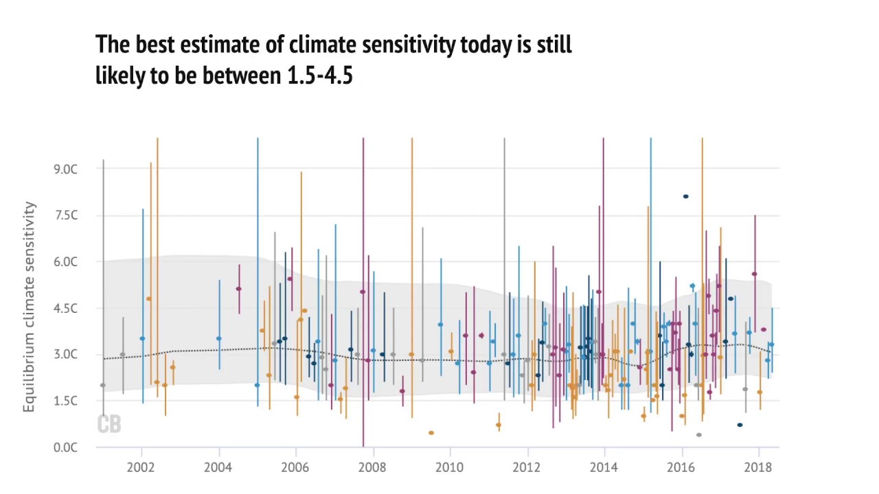
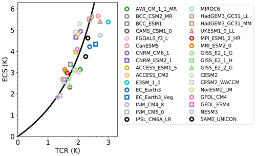
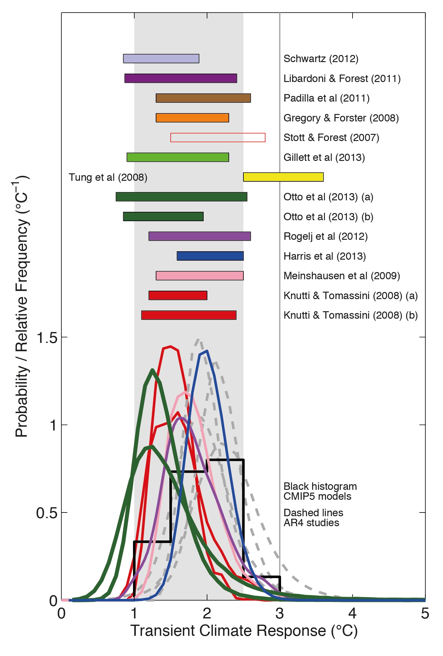

QUESTION: WHAT DOES UNCERTAINTY IN TCR AND ECS MEAN?
ANSWER: IT MEANS THAT THE CAUSAL RELATIONSHIP BETWEEN FOSSIL FUEL EMISSIONS AND TEMPERATURE THAT SITS AT THE HEART OF THE THEORY OF ANTHROPOGENIC GLOBAL WARMING IS EXPRESSED IN TERMS OF THESE TWO PARAMETERS BUT WE DON’T REALLY KNOW WHAT THEIR VALUES ARE.
QUESTION: WHAT DOES EMERGENT CONSTRAINT IN TCR AND ECS MEAN?
ANSWER: IT MEANS THAT ALTHOUGH WE DON’T KNOW WHAT THE ECS AND TCR SENSITIVITY VALUES ARE, WE DISCOVERED THAT THE DATA SINCE 1975 YIELD CONSISTENT AND STABLE VALUES FOR TCR AND ECS AND SO WE CAN USE THIS RANGE AS LIMITS WHEN ESTIMATING THESE PARAMETERS IN CLIMATE MODELS.
QUESTION: BUT CAN A THEORY DERIVED FROM THE DATA BE TESTED WITH THE SAME DATA? ISN’T THAT A KIND OF CIRCULAR REASONING?
ANSWER: YES, IT IS A FORM OF CIRCULAR REASONING CALLED THE TEXAS SHARPSHOOTER FALLACY WHERE YOU SHOOT FIRST AND DRAW THE TARGET CIRCLE LATER. THESE KINDS OF PROCEDURES, SUCH AS TESTING A HYPOTHESIS WITH THE SAME DATA USED TO CONSTRUCT THE HYPOTHESIS, ARE THE NORM IN CLIMATE SCIENCE WHERE STATISTICS EDUCATION IS AT A VERY LOW LEVEL.


QUESTION: HOW DO WE KNOW THAT STATISTICS EDUCATION IS AT A LOW LEVEL IN CLIMATE SCIENCE? WHAT IS THE EVIDENCE FOR THAT?
ANSWER: THERE ARE MANY EXAMPLES OF THAT IN CLIMATE SCIENCE THE MOST DRAMATIC BEING THE TCRE, TRANSIENT CLIMATE RESPONSE TO CUMULATIVE EMISSIONS. CORRELATIONS BETWEEN CUMULATIVE VALUES OF TIME SERIES DATA HAVE NO INTERPRETATION IN TERMS OF REAL WORLD PHENOMENA BECAUSE THESE CORRELATIONS ARE SPURIOUS. DETAILS OF THIS GROTESQUE FLAW IN CLIMATE SCIENCE ARE PROVIDED IN A RELATED POST ON THIS SITE. HERE IS THE LINK: https://tambonthongchai.com/2018/05/06/tcre/
ALSO THIS YOUTUBE VIDEO
AND THIS YOUTUBE VIDEO: In this Youtube video, one of the co-authors of the research paper cited above, demonstrates the use of circular reasoning to prove to climate activist Dir David Attenborough that humans are causing the current warming since pre-industrial times with their fossil fueled industrial economy as long as we move the pre-industrial date forward to “the 1970s” to make the data fit the hypothesis. The circular reasoning here is that a theory derived from the data cannot be tested with the same data.
ANOTHER EXAMPLE OF INADEQUATE STATISTICS EDUCATION IN CLIMATE SCIENCE IS THE INTERPRETATION OF UNCERTAINTY IN THAT DISCIPLINE. BRIEFLY, UNCERTAINTY DOES NOT MEAN OH! LOOK HOW HIGH IT COULD BE. IT MEANS WE DON’T REALLY KNOW. THE LESS WE KNOW THE HIGHER IT COULD BE AND IN PERFECT IGNORANCE IT COULD BE AS HIGH AS INFINITY BECAUSE THE ANSWER IS NOT CONSTRAINED BY INFORMATION.
The climate science view of uncertainty facilitates confirmation bias because the interpretation of the uncertain information can become biased by the beliefs, and activism priorities of the researcher.
THE UNCERTAINTY ISSUE IS DISCUSSED MORE FULLY IN A RELATED POST https://tambonthongchai.com/2020/04/22/climate-science-uncertainty/
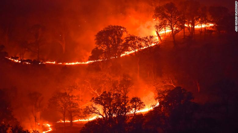

WHAT THE MEDIA SAYS
California has been hit by nearly 11,000 lightning strikes that have caused more than 367 known fires across the state in recent days, 26 of which are major. The state’s wildfire season is becoming much more destructive as climate change drives hotter and drier temperatures. (CNBC)
WHAT THE DATA SAYS


WITH THANKS TO PAUL HOMEWOOD AT ….
https://notalotofpeopleknowthat.wordpress.com/


DAMS AND SEA LEVEL RISE
Posted on: August 20, 2020

THIS POST IS A CRITICAL REVIEW OF A PAPER PUBLISHED IN NATURE ON THE IMPACT OF DAMS ON SEA LEVEL RISE.
CITATION: Frederikse, T., Landerer, F., Caron, L. et al. The causes of sea-level rise since 1900. Nature 584, 393–397 (2020). https://doi.org/10.1038/s41586-020-2591-3
ABSTRACT: The rate of global-mean sea-level rise since 1900 has varied over time, but the contributing factors are still poorly understood. Previous assessments found that the summed contributions of ice-mass loss, terrestrial water storage and thermal expansion of the ocean could not be reconciled with observed changes in global-mean sea level, implying that changes in sea level or some contributions to those changes were poorly constrained. Recent improvements to observational data, our understanding of the main contributing processes to sea-level change and methods for estimating the individual contributions, mean another attempt at reconciliation is warranted. Here we present a probabilistic framework to reconstruct sea level since 1900 using independent observations and their inherent uncertainties. The sum of the contributions to sea-level change from thermal expansion of the ocean, ice-mass loss and changes in terrestrial water storage is consistent with the trends and multidecadal variability in observed sea level on both global and basin scales, which we reconstruct from tide-gauge records. Ice-mass loss—predominantly from glaciers—has caused twice as much sea-level rise since 1900 as has thermal expansion. Mass loss from glaciers and the Greenland Ice Sheet explains the high rates of global sea-level rise during the 1940s, while a sharp increase in water impoundment by artificial reservoirs is the main cause of the lower-than-average rates during the 1970s. The acceleration in sea-level rise since the 1970s is caused by the combination of thermal expansion of the ocean and increased ice-mass loss from Greenland. Our results reconcile the magnitude of observed global-mean sea-level rise since 1900 with estimates based on the underlying processes, implying that no additional processes are required to explain the observed changes in sea level since 1900.
Estimating the sea-level budget: To obtain estimates of changes in global ocean mass (barystatic changes), we combine estimates of mass change for glaciers, ice sheets and terrestrial water storage (TWS). For the TWS estimate, we consider the effects of natural TWS variability, water impoundment in artificial reservoirs and groundwater depletion. For 2003–2018, we use observations from the Gravity Recovery and Climate Experiment (GRACE)29 to quantify the barystatic changes. We estimate changes in sea level due to global thermal expansion (thermosteric changes) from insitu subsurface observations30–32 over the period 1957–2018, and com-bine these estimates with an existing thermosteric reconstruction15. To obtain an estimate of GMSL changes and their accompanying uncertain-ties, we combine tide-gauge observations with estimates of local VLM from permanent Global Navigation Satellites System (GNSS) stations and with the difference between tide-gauge and satellite-altimetry observations.Each tide-gauge and VLM record is affected by glacial isostatic adjustment (GIA) and by the effects of gravity, rotation and deforma-tion (GRD) from contemporary surface-mass redistribution due to changes in ice mass and TWS. Owing to the irregular spatial distribution of tide-gauge sites, these effects could bias reconstructed global-mean and basin-mean sea-level changes33. To avoid this bias, we remove the local sea-level and VLM imprints from GIA and contemporary GRD effects from each tide-gauge and VLM record before computing basin-mean and global-mean sea-level changes from the tide gauges9.We propagate the uncertainties and associated covariances in the sea-level observations, in the contributing processes, and in the GIA and contemporary GRD effects into the final estimates of sea-level changes and the contributing processes. To this end, we generate an ensemble of 5,000 realizations of global-mean and basin-mean sea-level changes and all of the contributing processes. For processes for which multiple estimates are available, such as GIA, we randomly select one of these estimates when computing each individual ensemble member. For processes for which an estimate of the uncertainty is available, such as GNSS observations, we sample the estimate assuming a Gaussian distribution of the stated uncertainty about the corresponding mean. Then, we compute global-mean and basin-mean sea-level changes and the contributing processes for each ensemble member. We use the ensemble mean and spread to estimate all basin-mean and global-mean sea-level contributions and the associated confidence intervals. See Extended Data Fig.1 and Methods for a detailed description of our approach.Global-mean sea levelOur GMSL estimate (Fig.1a) shows a trend of 1.56±0.33mmyr−1 (90% confidence interval) over 1900–2018. It is also characterized by sub-stantial multidecadal variability, with higher rates of sea-level rise during the 1940s and since the 1990s, and lower rates around 1920 and 1970. The higher rates at the turn of the millennium are in good agreement with independent satellite-altimetry observations34. The observed trend over 1900–2018 is consistent with the sum of the esti-mated thermal expansion and changes in ocean mass, which sum to 1.52±0.33mmyr−1 (90% confidence interval). This consistency holds not only for the trends over the full study period, but also over the past 50 years (Table1), and for the pattern of multidecadal variability (Fig.1c), except for the low rates of sea-level change around the 1920s and early 1930s.Thermosteric and barystatic sea-level changes show similar multidec-adal variability patterns to the GMSL changes, although the amplitude of barystatic variability is larger than that of thermosteric variabil-ity, and barystatic variability is the main cause of multidecadal GMSL variability (Fig.1c). The barystatic variability is not dominated by a single process (Fig.1d). The above-average rate of GMSL rise in the 1940s is largely attributable to above-average contributions from glaciers and the Greenland Ice Sheet, whereas the high rate of barys-tatic sea-level rise since 2000 is attributable to both the Greenland and Antarctic ice sheets and to TWS. The low rates around 1970 are dominated by the TWS term (Fig.1d). This negative contribution is caused predominantly by reservoir impoundment.
CRITICAL COMMENTARY

Here, the assumption is that dam reservoirs sequester water from the land-ocean system such that land water that would have flowed to the ocean is captured and removed from the earth’s hydrological dynamics. If that were true we would have removed a cumulative amount of 300 gigatons of water by 1970 and 600 by 2010 as seen in the chart above. That corresponds to about 0.9mm of SLR equivalent by 1970 and 1.8 mm of SLR by 2010 or an annual SLR sequestration rate of 0.02mm of SLR lost to cumulative dam sequestration on an annual basis in the period 1930-2010.
However, dam reservoirs do not permanently remove water from the earth-ocean hydrological system but cause a delay in the transfer of the water through hydroelectricity and irrigation systems before the water is returned to the hydrological cycle and thereby to the ocean. However, the dams do delay the return of the water.
We estimate that the physical holdup in the reservoir is in the order of 12 days per billion cubic meters of reservoir capacity, but the the hydrological dynamics in the use of the water in terms of power generation, irrigation, and water supply to communities may delay the return of the water but this delay is unlikely to be more than seasonal or annual and certainly unlikely to be decadal or longer. More importantly, it is not possible for these effects to be cumulative.
However, it can be argued that at any given time the amount of water in the dams would otherwise have been in the ocean if it were not for dams and that they do represent an amount of sea level and that growth in dam reservoir capacity represents an equivalent sea level rise.
The diagram below shows that the effect of growth in dam reservoir capacity is estimated as 1.7mm of sea level over a period of 80 years. The corresponding rate of sea level rise is 0.02mm per year. This effect does not seem significant in the context of 3mm/year of AGW sea level rise particularly so in terms of a large uncertainty band of the SLR estimate in terms of global eustatic sea level in a dynamical system.