Archive for March 2020


[LINK TO THE HOME PAGE OF THIS SITE]
THIS POST IS A CRITICAL REVIEW OF ALARMING AGW DRIVEN GREENLAND ICE SHEET MELT REPORTED IN FORBES [LINK] AND CLIMATE HOME NEWS [LINK] WHERE THE CITED SOURCE IS AN IMBIE RESERCH PAPER [LINK] IMBIE STANDS FOR ICE SHEET MASS BALANCE INTER COMPARISON EXERCISE
PART-1: CLAIMS MADE IN THESE SOURCES
(1) THE FORBES SCIENCE ARTICLE “Greenland And Antarctica Are Melting Six Times Faster Than In The 1990s” [LINK] : Throughout the 1990s, Greenland and Antarctica together lost 81 billion tons of ice per year. But this month, a comprehensive assessment of the changing ice sheets published in the journal Nature, found that in the 2010s, the rate of ice loss has risen by a factor six. This means that the two ice sheets are now losing 475 billion tons of ice per year. The IPCC Fifth Assessment Report predicted a rise in global sea levels of 28 inches by 2100. But this new study shows that ice losses from both Antarctica and Greenland are rising faster than expected, tracking with the IPCC’s worst-case scenario. The Ice Sheet Mass Balance Intercomparison Exercise team, an international team of 89 polar scientists from 50 organizations, conducted the study. They combined 26 surveys to calculate changes in the mass of the Greenland and Antarctic ice sheets between 1992 and 2018, using data from 11 satellite missions, including measurements of the ice sheets’ changing volume, flow and gravity. The ice loss coincides with several years of intense surface melting in Greenland, including last summer’s Arctic heatwave, which means that 2019 is also likely to set a new record for polar ice sheet loss. Almost all of the ice lost from Antarctica and half of that lost from Greenland has been triggered by oceans melting their outlet glaciers, which causes them to speed up. The remainder of Greenland’s ice losses are due rising air temperature, which has melted the ice sheet at its surface.
(2) THE CLIMATE HOME ARTICLE: [LINK] Greenland ice loss much faster than expected. New results combine data from multiple satellite missions for an up-to-date assessment of changes across the ice-sheet. Between 1992 and 2017, Greenland lost 3.8 trillion tonnes of ice about seven times faster than expected. This corresponds to a 10.6 mm contribution to global sea-level rise. The Greenland ice sheet is losing mass seven times faster than in the 1990s, In a paper published today in Nature, an international team of 89 polar scientists, working in collaboration with ESA and NASA, have produced the most complete picture of Greenland ice loss to date. Over the study period, the rate of ice loss was found to have increased seven-fold from 33 billion tonnes per year 1990s to 254 billion tonnes per year in the last decade. The IMBIE teach combined data from 11 satellites including ESA’s ERS-1, ERS-2, Envisat and Cryosat missions, as well as the Copernicus Sentinel-1 and Sentinel-2 missions to monitor changes in the ice sheet’s volume, flow and gravity. Using observational data spanning three decades, the team has produced Greenland’s mass balance. This study condenses the available data and provides a consensus view regarding Greenland’s ice loss enabling more accurate projections of future sea rise to be made allowing coastal areas to prepare, and highlighting the urgent need for the international community to curtail greenhouse gas emissions. The IPCC had predicted a 60cm rise in global sea levels by 2100, putting 260 million people at risk of annual coastal flooding. The faster-than-expected rate reported by the IMBIE team shows that ice loss is following the IPCC’s high-end climate warming scenario, which predicts sea level will rise by an additional 7cm. For every 1cm rise in sea level, another six million people are exposed to coastal flooding. Greenland ice melt will cause 100 million people to be flooded each year by the end of the century. These changes will devastate coastal communities.” Climate models show that over half of the losses were because of increased surface meltwater runoff, driven by warming air temperatures. The remaining losses were the result of increased glacier flow triggered by rising ocean temperatures. Ice loss peaked at 335 gigatons/yr in 2011 dropping to an average of 238 gigatons/yr 2012- 2018 but still seven times higher than observed in the 1990s. The variable nature of the ice losses from Greenland over the last three decades (is a consequence of the wide range of physical processes affecting different sectors of the ice sheet and reflects the value of monitoring year-to-year fluctuations when attempting to close the global sea level budget. Greenhouse gas emissions are still going up, not down. We are leaving future generations to be confronted with increasingly severe impacts of climate change, such as rising sea levels. We need to redouble efforts to meet the internationally agreed goal to limit global warming to 1.5°C over pre-industrial levels.
(3) THE CITED RESEARCH PAPER: [LINK] Article: Published: 10 December 2019
Mass balance of the Greenland Ice Sheet from 1992 to 2018: The IMBIE Team
Nature volume 579, pages233–239(2020): Abstract: The Greenland Ice Sheet has been a major contributor to global sea-level rise in recent decades and it is expected to continue to be so. Although increases in glacier flow and surface melting have been driven by oceanic and atmospheric warming, the magnitude and trajectory of the ice sheet’s mass imbalance remain uncertain. Here we compare and combine 26 individual satellite measurements of changes in the ice sheet’s volume, flow and gravitational potential to produce a reconciled estimate of its mass balance. The ice sheet was close to a state of balance in the 1990s, but annual losses have risen since then, peaking at 345 ± 66 billion tonnes per year in 2011. In all, Greenland lost 3,902 ± 342 billion tonnes of ice between 1992 and 2018, causing the mean sea level to rise by 10.8 ± 0.9 mm. Using three regional climate models, we show that the reduced surface mass balance has driven 1,964 ± 565 billion tonnes (50.3 per cent) of the ice loss owing to increased meltwater runoff. The remaining 1,938 ± 541 billion tonnes (49.7 per cent) of ice loss was due to increased glacier dynamical imbalance, which rose from 46 ± 37 billion tonnes per year in the 1990s to 87 ± 25 billion tonnes per year since then. The total rate of ice loss slowed to 222 ± 30 billion tonnes per year between 2013 and 2017, on average, as atmospheric circulation favored cooler conditions and ocean temperatures fell at the terminus of Jakobshavn Isbræ. Cumulative ice losses from Greenland as a whole have been close to the rates predicted by the IPCC for their high-end climate warming scenario which forecast an additional 70 to 130 mm of global sea-level rise by 2100 compared with their central estimate.
PART-2: CRITICAL COMMENTARY
(1) THE ESSENTIAL FINDING OF THE CITED PAPER: The essential finding of the IMBIE team reported in this paper is that in the 27-year study period 1992 to 2018, Greenland lost 3,902 gigatonnes (GT) of ice. The corresponding annual rate is 144.52 GT/year. If this average rate sustains, the whole of the Greenland Ice Sheet (GIS) will be gone in 18,177.6 years raising global mean sea level (GMSL) by 7,360 mm 18,177.6 years from now at a rate of 0.405 mm/year. The corresponding sea level rise forecast for the year 2100 is 33.6 mm, well short of the IPCC & climate model forecast of 70 to 130 mm [LINK] . It is unlikely that the balance can be provided by Antarctica and other sources. These changes are implicitly attributed to AGW climate change and the fossil fuel emissions of the industrial economy with the implication that they can be moderated with climate action in the form of reducing emissions and eliminating the use of fossil fuels by moving the world’s energy infrastructure to renewables. The ice melt forecast at a millennial time scale will likely be interrupted by the next glaciation as we are now 12,000 years into the Holocene interglacial. The last interglacial, the Eemian, had lasted 15,000 years. It is therefore unlikely that the whole of the GIS will be melted by the Holocene. It is noted that the GIS had survived the Eemian interglacial considered by Paleo climatologists to have been a more violent ice-melt event than the Holocene [LINK]. Yet another consideration is that the paleo climate history of temperature variations in the last 12,000 years of the Holocene shows violent cycles of warming and cooling at millennial and centennial time scales [LINK] and therefore these trends cannot be extrapolated over millennia.
(2) SEARCHING FOR CALAMITY: It appears that the finding of a melt rate of 144.5 GT/year with corresponding GMSL rise of 0.405 mm/year was a disappointment to the IMBIE team who might have been looking in the data for something that would provide more alarming evidence of a “climate breakdown” or “climate emergency” or crisis that would serve as the rationale for costly climate action. It is likely for this reason that it became necessary for these scientists to review the data for a more creative presentation that could serve as an emergency with an urgent need for climate action. A look through the 27-year study period 1992-2018 revealed that if the mass balance time series is truncated at 2013, a higher annual average melt rate is found in the shorter 22-year time series 1992-2013. In this early portion of the data, the average annual melt rate is 254 GT/yr. At this rate, the whole of the GIS will be gone in 10,342 years raising sea levels by 0.712 mm/yr or 62.7mm by the year 2100. The corresponding forecast for the year 2100 is a sea level rise of 62.7mm, much closer to the IPCC and climate model forecast of 70 to 130 mm [LINK] with a reasonable possibility that the balance can be provided by Antarctica and other sources.
(3) CALAMITY FOUND: The large difference in mean annual melt rate between the 27-year time series (144 GT/yr) and the 22-year time series (254 GT/yr) likely provided the motivation for these scientists to rationalize the use of the shorter 22-year time series of melt data instead of the full span of the available data in the longer 27-year time series of melt data. A rationale was soon found. The scientists determined that the last 5-years of the full span of the data time series contains climate anomalies that must be removed from the data for a purely AGW climate change interpretation of the data. These anomalies are described as (1)Atmospheric circulation favored cooler conditions and ocean temperatures fell at the terminus of Jakobshavn Isbræ during the last 5 years of the sample period and (2)The melt rate is a closer fit to climate model and to IPCC forecasts when the last 5 years are removed from the data time series. Based on these considerations, the IMBIE scientists determined that the shorter time series 1992-2013 must be used to evaluate the impact of AGW climate change on the Greenland Ice Sheet / Accordingly, they determined that the Greenland Ice Sheet is being melted by AGW climate change at a rate of 254 GT/year and that this rate being consistent with the IPCC high emission scenario provides empirical evidence for the urgency of climate action to prevent sea level rise holocaust in the form of tidal floods in low lying regions of the world.
(4) ERRORS IN THE CALAMITY LOGIC OF IMBIE SCIENTISTS: ERROR#1: FORECAST STATISTICS: For making forecasts, we need as long a time series as possible as the basis for the forecast. In fact, the greater the variance in the data, the longer the data time series needs to be for the forecast being made to the year 2100. The high variance argument does not support the use of a shorter data time series for making the forecast to the year 2100. ERROR#2: CIRCULAR REASONING: A fundamental principle in statistics is that the data used to construct a hypothesis may not be used to test that hypothesis because that involves circular reasoning of the worst form best described as the TEXAS SHARPSHOOTER FALLACY [LINK] The circular reasoning used here are: (1)The shorter time series yields a higher average melt rate that better fits the theory and therefore it must be the better data set with which to test the theory. and (2)The shorter time series is a better fit to the IPCC forecast and therefore the lower melt rate in the longer time series must have an explanation in terms of climate and temperature anomalies and if we look for them we can surely find some climate and temperature anomalies to blame that on. ERROR#3: CIRCULAR REASONING. REDEFINING CALAMITY TO FIT THE DATA: In response to their failure to provide evidence of catastrophic sea level rise we had been told to fear, climate science has restructured sea level rise fear in terms of the few centimeters of SLR that they have evidence for, so that even low levels of sea level rise can be described as a climate change catastrophe. It is claimed that for every 10mm of sea level rise, 6 million people in low lying coastal areas are put at risk and that therefore we must cut fossil fuel emissions to save these people. This argument is weakened into irrelevance by two considerations. First, the cited study [LINK] uses eustatic mean sea level against DEM satellite data on coastal land elevation. These data contain a very high level of uncertainty that can create catastrophe out of nothing. Besides if there are only 6 million people for every 10mm rise in sea level, it would be much easier for the rest of the 7,800 million people of the world to take care of the unfortunate coastal lowland dwellers that too give up fossil fuels to reduce their high tide floods.

SUMMARY
The fear of AGW driven melt of the Greenland Ice Sheet and the resultant sea level rise presented in the IMBIE study cited above is not credible because the study suffers from methodological and statistical weaknesses in the form of circular reasoning. The idea, derived from uncertain satellite land elevation data that we should fear 10mm of sea level rise is yet another case of circular reasoning that says in effect that if we can’t find the sea level rise we fear we must fear the sea level rise we can find.
A further issue is that the large and incoherent variability of year to year ice melt may have a geothermal heat flux explanation as Greenland sits on a geologically active area as seen in a related post [LINK] . Rather than seek out parts of the time series with lower variance, the authors should study and attempt to understand the apparently random variability in year to year ice melt. A bibliography on geothermal heat under the Greenland ice sheet is provided below.
A second bibliography below implies that the failure to find catastrophic ice melt in Greenland this late in the Holocene may have to do with the finding that most of the interglacial effects on the GrIS have already occurred early in the Holocene. See also [LINK] .
BIBLIOGRAPHY: THE ROLE OF GEOTHERMAL HEAT IN GREENLAND
The studies below show significant impact of basal geothermal heat flux on ice melt
- Fahnestock, Mark, et al. “High geothermal heat flow, basal melt, and the origin of rapid ice flow in central Greenland.” Science 294.5550 (2001): 2338-2342. Age-depth relations from internal layering reveal a large region of rapid basal melting in Greenland. Melt is localized at the onset of rapid ice flow in the large ice stream that drains north off the summit dome and other areas in the northeast quadrant of the ice sheet. Locally, high melt rates indicate geothermal fluxes 15 to 30 times continental background. The southern limit of melt coincides with magnetic anomalies and topography that suggest a volcanic origin.
- Greve, Ralf. “Relation of measured basal temperatures and the spatial distribution of the geothermal heat flux for the Greenland ice sheet.” Annals of Glaciology 42 (2005): 424-432. The thermomechanical, three-dimensional ice-sheet model SICOPOLIS is applied to the Greenland ice sheet. Simulations over two glacial–interglacial cycles are carried out, driven by a climatic forcing interpolated between present conditions and Last Glacial Maximum anomalies. Based on the global heat-flow representation by Pollack and others (1993), we attempt to constrain the spatial pattern of the geothermal heat flux by comparing simulation results to direct measurements of basal temperatures at the GRIP, NorthGRIP, Camp Century and Dye 3 ice-core locations. The obtained heat-flux map shows an increasing trend from west to east, a high-heat-flux anomaly around NorthGRIP with values up to 135 mWm–2 and a low-heat-flux anomaly around Dye 3 with values down to 20 mW m–2. Validation is provided by the generally good fit between observed and measured ice thicknesses. Residual discrepancies are most likely due to deficiencies of the input precipitation rate and further variability of the geothermal heat flux not captured here.
- Greve, Ralf, and Kolumban Hutter. “Polythermal three-dimensional modelling of the Greenland ice sheet with varied geothermal heat flux.” Annals of Glaciology 21 (1995): 8-12. Computations over 50 000 years into steady state with Greve’s polythermal ice-sheet model and its numerical code are performed for the Greenland ice sheet with today’s climatological input (surface temperature and accumulation function) and three values of the geothermal heat flux: (42, 54.6, 29.4) mW m−2. It is shown that through the thermo-mechanical coupling the geometry as well as the thermal regime, in particular that close to the bed, respond surprisingly strongly to the basal thermal heat input. The most sensitive variable is the basal temperature field, but the maximum height of the summit also varies by more than ±100m. Furthermore, some intercomparison of the model outputs with the real ice sheet is carried out, showing that the model provides reasonable results for the ice-sheet geometry as well as for the englacial temperatures.
- van der Veen, Cornelis J., et al. “Subglacial topography and geothermal heat flux: Potential interactions with drainage of the Greenland ice sheet.” Geophysical research letters 34.12 (2007). Many of the outlet glaciers in Greenland overlie deep and narrow trenches cut into the bedrock. It is well known that pronounced topography intensifies the geothermal heat flux in deep valleys and attenuates this flux on mountains. Here we investigate the magnitude of this effect for two subglacial trenches in Greenland. Heat flux variations are estimated for idealized geometries using solutions for plane slopes derived by Lachenbruch (1968). It is found that for channels such as the one under Jakobshavn Isbræ, topographic effects may increase the local geothermal heat flux by as much as 100%.
- Dahl-Jensen, Dorthe, et al. “Past temperatures directly from the Greenland ice sheet.” Science 282.5387 (1998): 268-271. A Monte Carlo inverse method has been used on the temperature profiles measured down through the Greenland Ice Core Project (GRIP) borehole, at the summit of the Greenland Ice Sheet, and the Dye 3 borehole 865 kilometers farther south. The result is a 50,000-year-long temperature history at GRIP and a 7000-year history at Dye 3. The Last Glacial Maximum, the Climatic Optimum, the Medieval Warmth, the Little Ice Age, and a warm period at 1930 A.D. are resolved from the GRIP reconstruction with the amplitudes –23 kelvin, +2.5 kelvin, +1 kelvin, –1 kelvin, and +0.5 kelvin, respectively. The Dye 3 temperature is similar to the GRIP history but has an amplitude 1.5 times larger, indicating higher climatic variability there. The calculated terrestrial heat flow density from the GRIP inversion is 51.3 milliwatts per square meter.
- Petrunin, A. G., et al. “Heat flux variations beneath central Greenland’s ice due to anomalously thin lithosphere.” Nature Geoscience 6.9 (2013): 746-750. At the Earth’s surface, heat fluxes from the interior1 are generally insignificant compared with those from the Sun and atmosphere2, except in areas permanently blanketed by ice. Modelling studies show that geothermal heat flux influences the internal thermal structure of ice sheets and the distribution of basal melt water3, and it should be taken into account in planning deep ice drilling campaigns and climate reconstructions4. Here we use a coupled ice–lithosphere model driven by climate and show that the oldest and thickest part of the Greenland Ice Sheet is strongly influenced by heat flow from the deep Earth. We find that the geothermal heat flux in central Greenland increases from west to east due to thinning of the lithosphere, which is only about 25–66% as thick as is typical for terrains of early Proterozoic age5. Complex interactions between geothermal heat flow and glaciation-induced thermal perturbations in the upper crust over glacial cycles lead to strong regional variations in basal ice conditions, with areas of rapid basal melting adjoining areas of extremely cold basal ice. Our findings demonstrate the role that the structure of the solid Earth plays in the dynamics of surface processes.
- Brinkerhoff, Douglas J., et al. “Sensitivity of the frozen/melted basal boundary to perturbations of basal traction and geothermal heat flux: Isunnguata Sermia, western Greenland.” Annals of Glaciology 52.59 (2011): 43-50. A full-stress, thermomechanically coupled, numerical model is used to explore the interaction between basal thermal conditions and motion of a terrestrially terminating section of the west Greenland ice sheet. The model domain is a two-dimensional flowline profile extending from the ice divide to the margin. We use data-assimilation techniques based on the adjoint model in order to optimize the basal traction field, minimizing the difference between modeled and observed surface velocities. We monitor the sensitivity of the frozen/melted boundary (FMB) to changes in prescribed geothermal heat flux and sliding speed by applying perturbations to each of these parameters. The FMB shows sensitivity to the prescribed geothermal heat flux below an upper threshold where a maximum portion of the bed is already melted. The position of the FMB is insensitive to perturbations applied to the basal traction field. This insensitivity is due to the short distances over which longitudinal stresses act in an ice sheet.
- Tarasov, Lev, and W. Richard Peltier. “Greenland glacial history, borehole constraints, and Eemian extent.” Journal of Geophysical Research: Solid Earth 108.B3 (2003). We examine the extent to which observations from the Greenland ice sheet combined with three‐dimensional dynamical ice sheet models and semi‐Lagrangian tracer methods can be used to constrain inferences of the Eemian evolution of the ice sheet, of the extent and frequency of summit migration during the 100 kyr ice age cycle, and of the deep geothermal flux of heat from the Earth into the base of the ice sheet. Relative sea level, present‐day surface geometry, basal temperature, and age and temperature profiles from the Greenland Ice Project (GRIP) are imposed as constraints to tune ice sheet model and climate forcing parameters. Despite the paucity of observations, model‐based inferences suggest a significant northeast gradient in geothermal heat flux. Our analyses also suggest that during the glacial cycle, the contemporaneous summit only occupied the present‐day location during interglacial periods. On the basis of the development and use of a high‐resolution semi‐Lagrangian tracer analysis methodology for δ18O, we rule out isotropic flow disturbances due to summit migration as a possible source of the high Eemian variability of the GRIP δ18O record. Finally, in contrast with results obtained in some recent attempts to infer the extent to which Greenland may have contributed to the anomalous highstand of Eemian sea level, we find that conservative bounds for this contribution are 2–5.2 m, with a more likely range of 2.7–4.5 m.
BIBLIOGRAPHY : A HISTORY OF THE GREENLAND ICE SHEET
The bibliography shows that the significant changes to the GrIS expected from AGW climate change occurred early in the Holocene but not since then.
- Funder, Svend, et al. “The Greenland Ice Sheet during the past 300,000 years: A review.” Developments in Quaternary Sciences. Vol. 15. Elsevier, 2011. 699-713. The Greenland ice sheet‘s response to climate change is a major issue in the climate debate. This report reviews existing evidence on how the ice sheet margins reacted to climate change during the past 300,000 years—how it responded to the warm climate of the last interglacial and expanded on to the shelf during the last ice age. Compared to the other large ice sheets in the northern hemisphere, the Greenland ice sheet showed remarkable resilience to temperature change—a good omen for the future. [FULL TEXT].
- Ó Cofaigh, C., et al. “An extensive and dynamic ice sheet on the West Greenland shelf during the last glacial cycle.” Geology 41.2 (2013): 219-222. Considerable uncertainty surrounds the extent and timing of the advance and retreat of the Greenland Ice Sheet (GIS) on the continental shelf bordering Baffin Bay during the last glacial cycle. Here we use marine geophysical and geological data to show that fast-flowing ice sheet outlets, including the ancestral Jakobshavn Isbræ, expanded several hundred kilometers to the shelf edge during the last glaciation ca. 20 ka. Retreat of these outlets was asynchronous. Initial retreat from the shelf edge was underway by 14,880 calibrated (cal) yr B.P. in Uummannaq trough. Radiocarbon dates from the adjacent Disko trough and adjoining trough-mouth fan imply later deglaciation of Jakobshavn Isbræ, and, significantly, an extensive readvance and rapid retreat of this outlet during the Younger Dryas stadial (YD). This is notable because it is the first evidence of a major advance of the GIS during the YD on the West Greenland shelf, although the short duration suggests that it may have been out of phase with YD temperatures. [FULL TEXT]
- Jennings, Anne E., et al. “Paleoenvironments during Younger Dryas‐E arly Holocene retreat of the Greenland Ice Sheet from outer Disko Trough, central west Greenland.” Journal of Quaternary Science 29.1 (2014): 27-40. Paleo-environments during the late Younger Dryas through early Holocene retreat of the Greenland Ice Sheet from the outer shelf in the Disko Trough system of central West Greenland were investigated via lithofacies, foraminifera, dinocysts and sediment provenance analyses in radiocarbon‐dated sediment cores from the upper slope (JR175‐VC35) and outer shelf (JR175‐VC20 and HU2008029‐070CC). Core data show that the ice margin retreated rapidly from the outer shelf by calving, beginning by 12.2k cal a BP under cold paleoceanographic conditions with up to 11 months of sea‐ice. Ice retreat into Disko Bugt was well underway by 10.9k cal a BP. Enhanced ice‐sheet ablation in Disko Bugt and elsewhere along the West Greenland coast is inferred from cold glacial marine conditions associated with high sedimentation rates between 10.9 and 9.5k cal a BP on the outer shelf. Glacial marine conditions are recorded on the outer shelf until 7.8k cal a BP. Detrital carbonate‐bearing sediments rich in >2‐mm clasts deposited between 11.6 and 10.6 k cal a BP indicate that icebergs calved from northern Baffin Bay ice margins were melting and releasing sediments along West Greenland while the Greenland Ice Sheet margin was retreating into Disko Bugt. [FULL TEXT]
- Lecavalier, Benoit S., et al. “A model of Greenland ice sheet deglaciation constrained by observations of relative sea level and ice extent.” Quaternary Science Reviews 102 (2014): 54-84. An ice sheet model was constrained to reconstruct the evolution of the Greenland Ice Sheet (GrIS) from the Last Glacial Maximum (LGM) to present to improve our understanding of its response to climate change. The study involved applying a glaciological model in series with a glacial isostatic adjustment and relative sea-level (RSL) model. The model reconstruction builds upon the work of Simpson et al. (2009) through four main extensions: (1) a larger constraint database consisting of RSL and ice extent data; model improvements to the (2) climate and (3) sea-level forcing components; (4) accounting for uncertainties in non-Greenland ice. The research was conducted primarily to address data-model misfits and to quantify inherent model uncertainties with the Earth structure and non-Greenland ice. Our new model (termed Huy3) fits the majority of observations and is characterised by a number of defining features. During the LGM, the ice sheet had an excess of 4.7 m ice-equivalent sea-level (IESL), which reached a maximum volume of 5.1 m IESL at 16.5 cal ka BP. Modelled retreat of ice from the continental shelf progressed at different rates and timings in different sectors. Southwest and Southeast Greenland began to retreat from the continental shelf by ∼16 to 14 cal ka BP, thus responding in part to the Bølling-Allerød warm event (c. 14.5 cal ka BP); subsequently ice at the southern tip of Greenland readvanced during the Younger Dryas cold event. In northern Greenland the ice retreated rapidly from the continental shelf upon the climatic recovery out of the Younger Dryas to present-day conditions. Upon entering the Holocene (11.7 cal ka BP), the ice sheet soon became land-based. During the Holocene Thermal Maximum (HTM; 9-5 cal ka BP), air temperatures across Greenland were marginally higher than those at present and the GrIS margin retreated inland of its present-day southwest position by 40–60 km at 4 cal ka BP which produced a deficit volume of 0.16 m IESL relative to present. In response to the HTM warmth, our optimal model reconstruction lost mass at a maximum centennial rate of c. 103.4 Gt/yr. Our results suggest that remaining data-model discrepancies are affiliated with missing physics and sub-grid processes of the glaciological model, uncertainties in the climate forcing, lateral Earth structure, and non-Greenland ice (particularly the North American component). Finally, applying the Huy3 Greenland reconstruction with our optimal Earth model we generate present-day uplift rates across Greenland due to past changes in the ocean and ice loads with explicit error bars due to uncertainties in the Earth structure. Present-day uplift rates due to past changes are spatially variable and range from 3.5 to −7 mm/a (including Earth model uncertainty). [FULL TEXT]
- Larsen, Nicolaj K., et al. “Rapid early Holocene ice retreat in West Greenland.” Quaternary Science Reviews 92 (2014): 310-323. The possible demise of the Greenland ice sheet and its effect on global sea level rank among the most serious climate threats to society. To improve our knowledge about the future behaviour of the ice margin, we studied the ice sheet’s response to early Holocene warming in West Greenland using 47 cosmogenic 10Be exposure ages, 26 optically-stimulated luminescence ages as well as 15 new and 28 previously published radiocarbon ages. Paired bedrock and boulder ages show that the entire area was covered by warm-based ice during the Last Glacial Maximum (LGM), although glacial erosion was insufficient to completely remove the upper rock surface containing 10Be inherited from a previous period of exposure in bedrock samples above an elevation of 800 m. Our compilation of 10Be and 14C ages demonstrates that the ice sheet retreated from the outer-coast to the present ice margin between c. 11.4 and 10.4 cal. ka BP in the Godthåbsfjord system and between 10.7 ± 0.6 and 10.1 ± 0.4 ka ago in Buksefjord, whereas the coast at Sermilik became ice free at c. 10.5 cal. ka BP. We find no significant changes in the retreat rates between the deep Godthåbsfjord system and the Buksefjord-Sermilik region, which is characterized by only a few narrow and shallow fjords. However, deglaciation was initiated c. 700–900 years earlier in the Godthåbsfjord system indicating that the deep fjords probably triggered land-based deglaciation by dynamic ice loss leading to an overall rapid early Holocene ice retreat and drawdown of the ice sheet in West Greenland. These results demonstrate that even if there was a topographic control on the onset of deglaciation, fast ice retreat is not restricted to deep fjord systems but may occur independently of the topographic setting. [FULL TEXT]
- Young, Nicolás E., et al. “Age of the Fjord Stade moraines in the Disko Bugt region, western Greenland, and the 9.3 and 8.2 ka cooling events.” Quaternary Science Reviews 60 (2013): 76-90. Retreat of the western Greenland Ice Sheet during the early Holocene was interrupted by deposition of the Fjord Stade moraine system. The Fjord Stade moraine system spans several hundred kilometers of western Greenland’s ice-free fringe and represents an important period in the western Greenland Ice Sheet’s deglaciation history, but the origin and timing of moraine deposition remain uncertain. Here, we combine new and previously published 10Be and 14C ages from Disko Bugt, western Greenland to constrain the timing of Fjord Stade moraine deposition at two locations ∼60 km apart. At Jakobshavn Isfjord, the northern of two study sites, we show that Jakobshavn Isbræ advanced to deposit moraines ca 9.2 and 8.2–8.0 ka. In southeastern Disko Bugt, the ice sheet deposited moraines ca 9.4–9.0 and 8.5–8.1 ka. Our ice-margin chronology indicates that the Greenland Ice Sheet in two distant regions responded in unison to early Holocene abrupt cooling 9.3 and 8.2 ka, as recorded in central Greenland ice cores. Although the timing of Fjord Stade moraine deposition was synchronous in Jakobshavn Isfjord and southeastern Disko Bugt, within uncertainties, we suggest that Jakobshavn Isbræ advanced while the southeastern Disko Bugt ice margin experienced stillstands during the 9.3 and 8.2 ka events based on regional geomorphology and the distribution of 10Be ages at each location. The contrasting style of ice-margin response was likely regulated by site-specific ice-flow characteristics. Jakobshavn Isbræ’s high ice flux results in an amplified ice-margin response to a climate perturbation, both warming and cooling, whereas the comparatively low-flux sector of the ice sheet in southeastern Disko Bugt experiences a more subdued response to climate perturbations. Our chronology indicates that the western Greenland Ice Sheet advanced and retreated in concert with early Holocene temperature variations, and the 9.3 and 8.2 ka events, although brief, were of sufficient duration to elicit a significant response of the western Greenland Ice Sheet. [FULL TEXT]
- Roberts, David H., et al. “New constraints on Greenland ice sheet dynamics during the last glacial cycle: evidence from the Uummannaq ice stream system.” Journal of Geophysical Research: Earth Surface 118.2 (2013): 519-541. This paper presents the first assessment of the Uummannaq ice stream system (UISS) in West Greenland. The UISS drained ~6% of the Greenland ice sheet (GrIS) at the Last Glacial Maximum (LGM). The onset of the UISS is a function of a convergent network of fjords which feed a geologically controlled trough system running offshore to the shelf break. Mapping, cosmogenic radiogenic nuclide (CRN) dating, and model output reveal that glacially scoured surfaces up to 1266 m above sea level (asl) in fjord‐head areas were produced by warm‐based ice moving offshore during the LGM, with the elevation of warm‐based ice dropping westwards to ~700 m asl as the ice stream trunk zone developed. Marginal plateaux with allochthonous blockfields suggest that warm‐based ice produced till and erratics up to ~1200 m asl, but CRN ages and weathering pits suggest this was pre‐LGM, with only cold‐based ice operating during the LGM. Deglaciation began on the outer shelf at ~14.8 cal. kyrs B.P., with Ubekendt Ejland becoming ice free at ~12.4 ka. The UISS then collapsed with over 100 km of retreat by ~11.4 ka–10.8 cal. kyrs B.P., a rapid and complex response to bathymetric deepening, trough widening, and sea‐level rise coinciding with rapidly increasing air temperatures and solar radiation, but which occurred prior to ocean warming at ~8.4 cal. kyrs B.P. Local fjord constriction temporarily stabilized the unzipped UISS margins at the start of the Holocene before ice retreat inland of the current margin at ~8.7 ka. [FULL TEXT]
- Knutz, Paul C., et al. “Multiple‐stage deglacial retreat of the southern Greenland Ice Sheet linked with Irminger Current warm water transport.” Paleoceanography 26.3 (2011). There is limited knowledge pertaining to the history of the Greenland Ice Sheet (GIS) during the last glacial‐interglacial transition as it retreated from the continental margins to an inland position. Here we use multiproxy data, including ice‐rafted debris (IRD); planktonic isotopes; alkenone temperatures; and tephra geochemistry from the northern Labrador Sea, off southwest Greenland, to investigate the deglacial response of the GIS and evaluate its implications for the North Atlantic deglacial development. The results imply that the southern GIS retreated in three successive stages: (1) early deglaciation of the East Greenland margins, by tephra‐rich IRD that embrace Heinrich Event 1; (2) progressive retreat during Allerød culminating in major meltwater releases (δ18O depletion of 1.2‰) at the Allerød–Younger Dryas transition (12.8–13.0 kyr B.P.); and (3) a final stage of glacial recession during the early Holocene (∼9–11 kyr B.P.). Rather than indicating local temperatures of ambient surface water, the alkenones likely were transported to the core site by the Irminger Current. We attribute the timing of GIS retreat to the incursion of warm intermediate waters along the base of grounded glaciers and below floating ice shelves on the continental margin. The results lend support to the view that GIS meltwater presented a forcing factor for the Younger Dryas cooling. [FULL TEXT]
- Young, Nicolás E., et al. “Response of Jakobshavn Isbræ, greenland, to Holocene climate change.” Geology 39.2 (2011): 131-134. Rapid fluctuations in the velocity of Greenland Ice Sheet (GIS) outlet glaciers over the past decade have made it difficult to extrapolate ice-sheet change into the future. This significant short-term variability highlights the need for geologic records of preinstrumental GIS margin fluctuations in order to better predict future GIS response to climate change. Using 10Be surface exposure ages and radiocarbon-dated lake sediments, we constructed a detailed chronology of ice-margin fluctuations over the past 10 k.y. for Jakobshavn Isbræ, Greenland’s largest outlet glacier. In addition, we present new estimates of corresponding local temperature changes using a continuous record of insect (Chironomidae) remains preserved in lake sediments. We find that following an early Holocene advance just prior to 8 ka, Jakobshavn Isbræ retreated rapidly at a rate of ∼100 m yr−1, likely in response to increasing regional and local temperatures. Ice remained behind its present margin for ∼7 k.y. during a warm period in the middle Holocene with sustained temperatures ∼2 °C warmer than today, then the land-based margin advanced at least 2–4 km between A.D. 1500–1640 and A.D. 1850. The ice margin near Jakobshavn thus underwent large and rapid adjustments in response to relatively modest centennial-scale Holocene temperature changes, which may foreshadow GIS response to future warming.
THE HUMANS MUST SAVE THE PLANET
Posted on: March 30, 2020


AN ANTHROPOCENE LECTURE BY CLIMATE SCIENTIST MICHAEL MANN
[LINK TO THE HOME PAGE OF THIS SITE]
RELATED POST ON CLIMATE CHANGE ENVIRONMENTALISM: [LINK]
THE HISTORY, ORIGINS, AND THE IMPOSSIBILITY OF PLANETARY ENVIRONMENTALISM

(1) Historical roots of planetary environmentalism: The rapid industrial and economic growth in the post-war era progressed mostly without adequate safeguards against environmental degradation. This situation became sensationalized through a series of high profile events that captured public attention. The wanton use of pesticides such as DDT was blamed for killing butterflies and birds (Carson, 1962). The explosive growth in automobile ownership shrouded large cities like Los Angeles and New York in smog (Gardner, 2014) (Haagen-Smit, 1952) (Hanst, 1967). The widespread dumping of industrial waste into lakes and rivers was highlighted by events such as the fire in the Cuyahoga River (Marris, 2011) (Goldberg, 1979).
(2) The hippie counter-culture movement of the 1960s rejected many conventional values and in particular, the assumed primacy of technological advancement and industrial growth. It opposed the unrestricted use of pesticides, herbicides, preservatives, food additives, fertilizers, and other synthetic chemicals. It fought against the release of industrial waste into the atmosphere and into waterways, the harvesting of old growth forests for the wood and paper industries, and the inadequacy of public transit that could limit the number of automobiles in big cities and the air pollution they cause (Rome, 2003) (Zelko, 2013).
(3): This environmental movement was the driving force behind the formation of the Environmental Protection Agency (EPA) in the USA which was given the laws, the ways, the means, and the power to act quickly and decisively to clean up the air and water(Ruckelshaus, 1984). In Canada, a Ministry of Environment was created with the same mandate. It has since been renamed as the Ministry of Environment and Climate Change.
The EPA cleaned up the air and the water in the USA with strictly enforced new laws and procedures that limited the concentration of harmful chemicals in all industrial effluents and also required all new enterprises to obtain the approval of the EPA of their environmental impact before they could proceed. The remarkable success of the EPA made it a model for environmental law and environmental protection in countries around the world (Ruckelshaus, 1984) (Andreen, 2004) (Dolin, 2008).
(4) THE EXTENSION OF ENVIRONMENTALISM TO THE BAMBI PRINCIPLE Environmentalism in its conceptual sense is the idea that humans should take care of the environment for their own good such that human life, health, and security are enhanced. This idea is contained in the hippie wisdom that if you shit in bed you will sleep in shit. At some point, the enthusiasm of environmentalism became separated from this fundamental reality and the conceptual underpinnings of environmentalism were arbitrarily extended in a spirit of emotional enthusiasm into what we can call “Tree Hugger” environmentalism” or the “The Bambi Principle” discussed in a related post on this site: LINK: [THE BAMBI PRINCIPLE] in which the concept of environmentalism became corrupted first by separating humans from nature and second with a role for humans as caretakers of nature. It meant that humans must take care not only of their environment but of nature itself such that humans now saw themselves as caretakers of nature. THESE ANOMALIES IN ENVIRONMENTALISM HAVE LED ANALYSTS TO PROPOSE THAT ENVIRONMENTALISM IS THE NEW RELIGION OF THE POST MODERN WORLD: [LINK]
(5) A GLOBAL REACH; It was also found that industrial waste in rivers draining into the ocean was having detrimental effects on oceanic biota and chemistry such that fundamental oceanic properties now seemed threatened by human activity. It was thus that the “environment” to be taken care of became extended to include the entire crust of the planet including the land and the ocean and all the creatures big and small that live there. In essence man became nature’s manager and keeper. Environmentalism now meant more than man making sure his environment will sustain him. It meant that man was now in charge of nature. This is the conceptual bridge that when extended to the planetary scale led to the idea of the Anthropocene that gave man a godlike role on the planet earth consistent with his Bibilical Dominion over the Beasts.
(6) PICTURES FROM SPACE AND THE EXTENSION OF ENVIRONMENTALISM TO THE PLANET


It was about then, late in the year 1972, that the first picture of the planet was taken from space and flashed on TV screens around the world. The picture was taken by the crew of the Apollo-9 space craft. This image created an overwhelming sense of awe as well as a sense of insecurity to see the finite little thing that we live on that had seemed so infinitely big as viewed from the surface instead of from space.
(7) PLANETARY ENVIRONMENTALISM: This image caused a profound change in environmentalism such that our “environment” became redefined as the planet itself. It is thus that the “environment” of environmentalism underwent a grand and dramatic change. In the new planetary context of environmentalism, our environment is the same wherever we are and it is the whole of the planet earth. For example, the environment I live in is not just the rice fields and sugar palms of Phetchaburi, but the whole of the planet earth.


(8) THE RISE OF PLANETARY ENVIRONMENTALISM This image from space encouraged environmentalists to look at wider impacts of pollution and they quickly learned that both water pollution carried by rivers to the ocean and air pollution anywhere on earth have a reach much larger than they had imagined. For example ocean pollution in Southeastern USA could be carried by ocean currents thousands of miles away where it could have a detrimental impact. And air pollution in Corsica could affect air quality in Athens; and environmentalist James Lovelock found long lived chlorofluorocarbon (CFC) compounds used in refrigerants and hairspray in the atmosphere in the middle of the Atlantic Ocean. Environmentalism thus became global and soon thereafter, environmental scientists Sherwood Rowland and Mario Molina of UC Irvine proposed a theory that the long life of CFC discovered by Lovelock implies that these chemicals could eventually end up in the stratosphere where they could act as catalytic agents of ozone destruction. The United Nations entered the scene to take charge of global environmental issues by forming the United Nations Environmental Program (UNEP) and immediately went to work on the global environmental problem of ozone depletion implied by the works of Sherwood Rowland and Mario Molina. Environmentalism was now planetary and the UN bureaucracy had automatically extended itself and its budget in its new UNEP role as a Global Environmental Protection Agency that can address global environmental issues.


(9) PLANETARY ENVIRONMENTALISM AND THE ROLE OF HUMANS AS CARETAKERS OF THE PLANET EARTH IN THE ANTHROPOCENE. In his paper “Geology of Mankind”, geologist Paul Crutzen calls on geologists to use the term ‘Anthropocene’ for the current “human-dominated” geological epoch, that sits piggy-back on the Holocene [LINK] . Since then there have been a number of papers, mostly by Will Steffen, on the Anthropocene as seen in the bibliography below. A succinct summary of this concept is provided by Noam Chomsky in the video below. It describes a state of the world in which humans are in control of the planet and are now its keepers and caretakers. The fate of the planet now depends on how well humans take care of it. This is the extent to which global environmentalism has been taken and and the context in which the ozone crisis and the climate crisis of our time should be understood.
(10) THE IMPOSSIBILITY OF PLANETARY ENVIRONMENTALISM: Here we argue that the concept of the Anthropocene and of human caused planetary catastrophe by way of things like the industrial economy running on fossil fuels are inconsistent with the relative insignificance of humans on a planetary scale. Consider for example, that even as humans are worried about things like carbon pollution and the population bomb in terms of the planet being overwhelmed by the sheer number of humans on earth, humans, like all life on earth, are carbon life forms created from the carbon that came from the mantle of the planet but a rather insignificant portion of it. In terms of total weight, humans constitute 0.05212% of the total mass of life on earth. Yet we imagine that our numbers are so huge that the planet will be overwhelmed by our population bomb. All the life on earth taken together is 0.000002875065% of the crust of the planet by weight. The crust of the planet we see in the pictures from space and where we live and where we have things like land, ocean, atmosphere, climate, and carbon life forms, is 0.3203% of the planet by weight. The other 99.6797% of the planet, the mantle and core, is a place where we have never been and will never be and on which we have no impact whatsoever. In terms of the much feared element carbon that is said to cause planetary devastation by way of climate change and ocean acidification, a mass balance shows that the crust of the planet where we live contains 0.201% of the planet’s carbon with the other 99.8% of the carbon inventory of the planet being in the mantle and core.
OUR BIBLICAL DOMINION OVER NATURE
(11) THE CONCLUSION WE DRAW FROM THIS MASS BALANCE ANALYSIS IS THAT:
- The crust of the planet where we live is an insignificant portion of the planet.
- Life on earth is an insignificant portion of the crust of the planet.
- Humans are an insignificant portion of life on earth.
Although it is true that humans must take care of their environment, we propose that the environment should have a more rational definition because the mass balance above does not show that humans are a significant force on a planetary scale or that they are in a position to either save it or to destroy it even with the much feared power of their fossil fueled industrial economy. And that implies that it is not possible that there is such a thing as an Anthropocene in which humans are the dominant geological force of the planet.
Like ants and bees, humans are social creatures that live in communities of humans so that when they look around all they see are humans. This is the likely source of our human oriented view of the world. Paul Ehrlich’s overpopulation theory is derived from his first visit to India which he described as “people people people people people!” It is this biased view of the planet that makes it possible for us to extrapolate Calcutta to the planet and come up with the fearful image described by Jeff Gibbs as “Have you every wondered what would happen if a single species took over an entire planet?”
RELATED POSTS
- THE ISSUE IS FOSSIL FUELS NOT CLIMATE CHANGE: [LINK]
- NO EVIDENCE THAT ATMOSPHERIC COMPOSITION IS RESPONSIVE TO FOSSIL FUEL EMISSIONS: [LINK]
- NO EVIDENCE THAT SURFACE TEMPERATURE IS RESPONSIVE CUMULATIVE FOSSIL FUEL EMISSIONS AS CLAIMED IN THE “TRANSIENT CLIMATE RESPONSE TO CUMULATIVE EMISSIONS” [LINK]
- NO EVIDENCE THAT CLIMATE ACTION WILL CHANGE THE RATE OF WARMING: [LINK]
- THE UNABOMBER’S MOVEMENT AGAINST THE INDUSTRIAL ECONOMY: [LINK]


ANTHROPOCENE BIBLIOGRAPHY
- Anthropocene doomsday scenario: Steffen 2018: Steffen, Will, et al. “Trajectories of the Earth System in the Anthropocene.” Proceedings of the National Academy of Sciences (2018): 201810141. {We explore the risk that self-reinforcing feedbacks could push the Earth System toward a planetary threshold that, if crossed, could prevent stabilization of the climate at intermediate temperature rises and cause continued warming on a “Hothouse Earth” pathway even as human emissions are reduced. Crossing the threshold would lead to a much higher global average temperature than any interglacial in the past 1.2 million years and to sea levels significantly higher than at any time in the Holocene. We examine the evidence that such a threshold might exist and where it might be. If the threshold is crossed, the resulting trajectory would likely cause serious disruptions to ecosystems, society, and economies. Collective human action is required to steer the Earth System away from a potential threshold and stabilize it in a habitable interglacial-like state. Such action entails stewardship of the entire Earth System—biosphere, climate, and societies—and could include decarbonization of the global economy, enhancement of biosphere carbon sinks, behavioral changes, technological innovations, new governance arrangements, and transformed social values.}
- Anthropocene doomsday scenario: Steffen 2015: Steffen, Will, et al. “The trajectory of the Anthropocene: the great acceleration.” The Anthropocene Review 2.1 (2015): 81-98. {The ‘Great Acceleration’ graphs, originally published in 2004 to show socio-economic and Earth System trends from 1750 to 2000, have now been updated to 2010. In the graphs of socio-economic trends, where the data permit, the activity of the wealthy (OECD) countries, those countries with emerging economies, and the rest of the world have now been differentiated. The dominant feature of the socio-economic trends is that the economic activity of the human enterprise continues to grow at a rapid rate. However, the differentiated graphs clearly show that strong equity issues are masked by considering global aggregates only. Most of the population growth since 1950 has been in the non-OECD world but the world’s economy (GDP), and hence consumption, is still strongly dominated by the OECD world. The Earth System indicators, in general, continued their long-term, post-industrial rise, although a few, such as atmospheric methane concentration and stratospheric ozone loss, showed a slowing or apparent stabilisation over the past decade. The post-1950 acceleration in the Earth System indicators remains clear. Only beyond the mid-20th century is there clear evidence for fundamental shifts in the state and functioning of the Earth System that are beyond the range of variability of the Holocene and driven by human activities. Thus, of all the candidates for a start date for the Anthropocene, the beginning of the Great Acceleration is by far the most convincing from an Earth System science perspective.}
- Anthropogenic doomsday scenario: McGill 2015 : McGill, Brian J., et al. “Fifteen forms of biodiversity trend in the Anthropocene.” Trends in ecology & evolution 30.2 (2015): 104-113. {Humans are transforming the biosphere in unprecedented ways, raising the important question of how these impacts are changing biodiversity. Here we argue that our understanding of biodiversity trends in the Anthropocene, and our ability to protect the natural world, is impeded by a failure to consider different types of biodiversity measured at different spatial scales. We propose that ecologists should recognize and assess 15 distinct categories of biodiversity trend. We summarize what is known about each of these 15 categories, identify major gaps in our current knowledge, and recommend the next steps required for better understanding of trends in biodiversity.}
- Anthropocene doomsday scenario: Dirzo, 2014 : Dirzo, Rodolfo, et al. “Defaunation in the Anthropocene.” science 345.6195 (2014): 401-406. {We live amid a global wave of anthropogenically driven biodiversity loss: species and population extirpations and, critically, declines in local species abundance. Particularly, human impacts on animal biodiversity are an under-recognized form of global environmental change. Among terrestrial vertebrates, 322 species have become extinct since 1500, and populations of the remaining species show 25% average decline in abundance. Invertebrate patterns are equally dire: 67% of monitored populations show 45% mean abundance decline. Such animal declines will cascade onto ecosystem functioning and human well-being. Much remains unknown about this “Anthropocene defaunation”; these knowledge gaps hinder our capacity to predict and limit defaunation impacts. Clearly, however, defaunation is both a pervasive component of the planet’s sixth mass extinction and also a major driver of global ecological change.}
- Anthropocene doomsday scenario: Braje 2013 : Braje, Todd J., and Jon M. Erlandson. “Human acceleration of animal and plant extinctions: A Late Pleistocene, Holocene, and Anthropocene continuum.” Anthropocene 4 (2013): 14-23. {One of the most enduring and stirring debates in archeology revolves around the role humans played in the extinction of large terrestrial mammals (megafauna) and other animals near the end of the Pleistocene. Rather than seeking a prime driver (e.g., climate change, human hunting, disease, or other causes) for Pleistocene extinctions, we focus on the process of human geographic expansion and accelerating technological developments over the last 50,000 years, changes that initiated an essentially continuous cascade of ecological changes and transformations of regional floral and faunal communities. Human hunting, population growth, economic intensification, domestication and translocation of plants and animals, and landscape burningand deforestation, all contributed to a growing human domination of earth’s continental and oceanic ecosystems. We explore the deep history of anthropogenic extinctions, trace the accelerating loss of biodiversity around the globe, and argue that Late Pleistocene and Holocene extinctions can be seen as part of a single complex continuum increasingly driven by anthropogenic factors that continue today.}
- Anthropocene doomsday scenario: Steffen 2011: Steffen, Will, et al. “The Anthropocene: From global change to planetary stewardship.” Ambio 40.7 (2011): 739. {Over the past century, the total material wealth of humanity has been enhanced. However, in the twenty-first century, we face scarcity in critical resources, the degradation of ecosystem services, and the erosion of the planet’s capability to absorb our wastes. Equity issues remain stubbornly difficult to solve. This situation is novel in its speed, its global scale and its threat to the resilience of the Earth System. The advent of the Anthropence, the time interval in which human activities now rival global geophysical processes, suggests that we need to fundamentally alter our relationship with the planet we inhabit. Many approaches could be adopted, ranging from geo-engineering solutions that purposefully manipulate parts of the Earth System to becoming active stewards of our own life support system. The Anthropocene is a reminder that the Holocene, during which complex human societies have developed, has been a stable, accommodating environment and is the only state of the Earth System that we know for sure can support contemporary society. The need to achieve effective planetary stewardship is urgent. As we go further into the Anthropocene, we risk driving the Earth System onto a trajectory toward more hostile states from which we cannot easily return.}
- Anthropocene doomsday scenario: Wagler 2011 : Wagler, Ron. “The anthropocene mass extinction: An emerging curriculum theme for science educators.” The American Biology Teacher 73.2 (2011): 78-83. {There have been five past great mass extinctions during the history of Earth. There is an ever-growing consensus within the scientific community that we have entered a sixth mass extinction. Human activities are associated directly or indirectly with nearly every aspect of this extinction. This article presents an overview of the five past great mass extinctions; an overview of the current Anthropocene mass extinction; past and present human activities associated with the current Anthropocene mass extinction; current and future rates of species extinction; and broad science-curriculum topics associated with the current Anthropocene mass extinction that can be used by science educators. These broad topics are organized around the major global, anthropogenic direct drivers of habitat modification, fragmentation, and destruction; overexploitation of species; the spread of invasive species and genes; pollution; and climate change.}
- Anthropocene doomsday scenario: Zalasiewicz 2010 : Zalasiewicz*, Jan, et al. “The new world of the Anthropocene.” (2010): 2228-2231. {Global events such as mass extinctions, the onset of Ice Ages, and changes in geochemistry linked with changes in atmospheric chemistry are timeposts in geological strata. In the timeline for Earth history, they allow segmentation of its 4.6 billion year existence into eons, eras, periods, and epochs. As human activity makes its recently initiated yet globally extensive mark that is leading to mass extinctions, changes in atmospheric and marine chemistry, and altering terrestrial features, should a new epoch be declared? Can such an Anthropocene be geologically standardized in strata? Zalasiewicz et al make their case in this article featured in ES&T’s April 1, 2010 print issue recognizing the 40th Anniversary of Earth Day.}
- Anthropocene doomsday scenario: Saxon 2008 : Saxon, Earl. “Noah’s Parks: A partial antidote to the Anthropocene extinction event.” Biodiversity 9.3-4 (2008): 5-10. {Climate change will rapidly alter the abiotic environment of many localities leading to significant losses of biodiversity in ecosystems unable to adapt quickly. However, local extirpation will be least likely where environmental change is slowest. Such locations will offer refugia for species with narrow environmental ranges, provide persistent sources of colonists, offer transitory homes for dispersers and serve as platform sites on which new community assemblages develop. Consequently, networks of protected areas that include such sites will conserve more biodiversity. Conventional protected area network selection algorithms give priority to areas with the lowest current cost. I added projected environmental change as a cost factor. I applied the modified algorithm in three arctic ecoregions where climate change is predicted to be extremely rapid and to 20 tropical ecoregions where the pace of climate change will be slower but many species are vulnerable to small changes. I identified protected area networks that protect places where change will be slowest in all ecoregions. These climate-adaptive protected area networks differ substantially from both current protected area networks and near-optimal networks that are based only on current costs. The modified method will help protected area planners to acquire potential climate refugia and to help implement adaptive conservation strategies for potential refugia that are already protected. It will also help reduce the risk that projected refugia are unknowingly allocated to land uses incompatible with their critical role in biodiversity conservation.}
- Anthropocene doomsday scenaro: Steffen 2007: Steffen, Will, Paul J. Crutzen, and John R. McNeill. “The Anthropocene: are humans now overwhelming the great forces of nature.” AMBIO: A Journal of the Human Environment 36.8 (2007): 614-621. {We explore the development of the Anthropocene, the current epoch in which humans and our societies have become a global geophysical force. The Anthropocene began around 1800 with the onset of industrialization, the central feature of which was the enormous expansion in the use of fossil fuels. We use atmospheric carbon dioxide concentration as a single, simple indicator to track the progression of the Anthropocene. From a preindustrial value of 270–275 ppm, atmospheric carbon dioxide had risen to about 310 ppm by 1950. Since then the human enterprise has experienced a remarkable explosion, the Great Acceleration, with significant consequences for Earth System functioning. Atmospheric CO2 concentration has risen from 310 to 380 ppm since 1950, with about half of the total rise since the preindustrial era occurring in just the last 30 years. The Great Acceleration is reaching criticality. Whatever unfolds, the next few decades will surely be a tipping point in the evolution of the Anthropocene.}


THE CORRUPTION OF EDUCATION WITH CLIMATE ACTIVISM
STATEMENT BY COLUMBIANEWS@COLUMBIA.EDU: How Should Columbia Drive Climate Change Innovation? The University asks students to collaborate on building a road map for climate response and a more sustainable future. Published by columbianews@columbia.edu November 15, 2019.
As the climate crisis mounts, Columbia has turned to its students for ideas and partnership in addressing one of the most critical global challenges of our times. On Nov. 8 and 11, the University held two Climate Town Hall discussions to explore ways in which students can help set a trajectory for Columbia’s climate response that will serve as a model for higher education. The student forums are an outgrowth of the Climate Change Task Force announced by President Lee C. Bollinger in September. Led by Alex Halliday, director of Columbia’s Earth Institute, the 24-member task force represents diverse disciplines, from the arts and humanities to the natural and social sciences.
STUDENT CLIMATE TOWN HALLS
Nov. 8 Town Hall Forum, Nov. 11 Town Hall Forum
“With the seminal and superb science being carried out at the Lamont-Doherty Earth Observatory, as well as across the University broadly, brought together through the Earth Institute, Columbia has been, and is, at the very forefront of academic discovery related to climate change” said President Bollinger in an email announcing the task force to the community. “Yet, it is important that we ask, as one of the leading universities in the world: Are we doing enough?” In addressing a group of about 60 students who attended the Nov. 11 town hall (a similar number attended the first event), Halliday said he wanted the students to feel empowered. “I’m looking for your ideas,” he said. “We really want to hear what you think Columbia could—or should—be doing in the area of upping its game in the battle against climate change or making a bigger effect on society in a way that would scale quite significantly and help us move the dial on the issue.” About 20 students spoke at each forum, offering ideas that ranged from innovative clean-energy solutions to improved climate education to hands-on support for students choosing environmental and sustainability career pathways.
Some of the ideas generated at the Town Hall:
Shore up silos in schools, institutes and across disciplines in an overarching climate school or consortium. Tackling climate change requires cross-disciplinary research, engagement, initiatives and perspectives that include science, art, medicine, architecture, psychology, journalism, the social sciences and more. Create a Climate Café to involve students, faculty, staff and the public in the climate conversation. The venue could serve as a hub for sharing knowledge and ideas and foster collaborative efforts. Include more climate science modules in existing courses, create new climate-focused classes and make climate study a pillar of Columbia’s Core Curriculum, the set of common courses required of all undergraduates. Develop continuing education climate courses to expose a broader audience to climate education and expand the University’s reach and impact. Strengthen course offerings to high school students who participate in Columbia summer programs. Reduce the University’s carbon footprint even further. Suggested initiatives include refitting buildings to be more energy-efficient, adding compost bins, reconsider maintaining the greenery of campus lawns and installing additional bike racks. Divest from all fossil fuel investments. (In 2017, the Columbia Board of trustees voted to divest from thermal coal producers.) Provide incentives for students to represent the University as climate communicators, such as academic credit to visit New York City schools and community events or providing funding to attend global meetings, such as the United Nations Conference on Climate Change. Connect green-tech entrepreneurs to the Columbia research community and promote solutions developed by engineering faculty and others to platforms that can bring green-technology innovations into the world. Expand the University’s role in educating students about environmental and sustainability career pathways. Set up mechanisms that connect students to professional opportunities in industry, government, education and nonprofits. The Climate Change Task Force is scheduled to submit a 200-page report to President Bollinger and the trustees by Dec. 1 that catalogs ongoing sustainability efforts across Columbia with recommendations for the future.
SEE ALSO
[EARTH INSTITUTE1] [COLUMBIA CLIMATE CENTER] [EARTH INSTITUTE2]
POSTS AT THIS SITE THAT IMPLY CLIMATE ACTIVISM AT COLUMBIA
RELATED POST ON JOURNALISM AT COLUMBIA UNIVERSITY: [LINK]
RELATED POST#1 ON THE MONTREAL PROTOCOL AS A MODEL FOR GLOBAL ACTION ON CLIMATE [LINK]
RELATED POST#2 ON THE MONTREAL PROTOCOL AS MODEL FOR GLOBAL ACTION ON CLIMATE [LINK]
RELATED POST ON THE CURRENT WARMING PERIOD AS “UNPRECEDENTED” [LINK]
RELATED POST ON AGW CLIMATE CHANGE AND ICE SHELF COLLAPSE IN ANTARCTICA [LINK]
CONCLUSION: COLUMBIA UNIVERSITY IS NOT A RELIABLE AND UNBIASED SOURCE OF CLIMATE RESEARCH FINDINGS BECAUSE OF ITS INVOLVEMENT IN CLIMATE ACTIVISM. THEREFORE, PUBLICATIONS OF THE EARTH INSTITUTE OF COLUMBIA UNIVERSITY AND CLIMATE RESEARCH PAPERS BY COLUMBIA UNIVERSITY ACADEMICS MUST BE INTERPRETED IN THIS LIGHT BECAUSE THEY CANNOT BE ASSUMED TO BE UNBIASED SCIENTIFIC INQUIRY.

THE OZONE MYSTERY DEEPENS
Posted on: March 27, 2020

[LINK TO THE HOME PAGE OF THIS SITE]
RELATED POST ON THIS TOPIC: [LINK]
RELATED POSTS ON OZONE DEPLETION: [LINK] [LINK] [LINK] [LINK]
RELATED POSTS ON COLUMBIA UNIVERSITY [LINK]
SCIENCE ALERT MAGAZINE ARTICLE 26 MARCH 2020: Earth’s Ozone Layer Is Healing and Bringing Some Good News on Global Wind Movement, CARLY CASSELLA, 26 MARCH 2020
The ozone layer above Antarctica has recovered so much, it’s actually stopped many worrying changes in the Southern Hemisphere’s atmosphere. If you’re looking for someone to thank, try the world at large. A new study suggests the Montreal Protocol – the 1987 agreement to stop producing ozone depleting substances (ODSs) – could be responsible for pausing, or even reversing, some troubling changes in air currents around the Southern Hemisphere. Swirling towards our planet’s poles at a high altitude are fast air currents known as jet streams. Before the turn of the century, ozone depletion had been driving the southern jet stream further south than usual. This ended up changing rainfall patterns, and potentially ocean currents as well. Then, a decade or so after the protocol was signed, that migration suddenly stopped.
Was it a coincidence? Using a range of models and computer simulations, researchers have now shown this pause in movement was not driven by natural shifts in winds alone. Instead, only changes in the ozone could explain why the creep of the jet stream had suddenly stopped. In other words, the impact of the Montreal Protocol appears to have paused, or even slightly reversed, the southern migration of the jet stream. And for once, that’s actually good news.
In Australia, for instance, changes to the jet stream have increased the risk of drought by pushing rain away from coastal areas. If the trend does reverse, those rains might return.
“The ‘weather bands’ that bring our cold fronts have been narrowing towards the south pole, and that’s why southern Australia has experienced decreasing rainfall over the last thirty years or so,” says Ian Rae, organic chemist from the University of Melbourne who was not involved in the study. “If the ozone layer is recovering, and the circulation is moving north, that’s good news on two fronts (pun not intended).”
Still, we may not be celebrating for long. While improvements in cutting back our reliance on ODSs have certainly allowed the ozone to recover somewhat, carbon dioxide levels continue to creep upwards and place all that progress at risk.
Last year, the Antarctic ozone hole hit its smallest annual peak on record since 1982, but the problem isn’t solved, and this record may have something to do with unusually mild temperatures in that layer of the atmosphere. What’s more, in recent years, there’s been a surge in ozone-depleting chemicals, coming from industrial regions in China.
“We term this a ‘pause’ because the poleward circulation trends might resume, stay flat, or reverse,” says atmospheric chemist Antara Banerjee from the University of Colorado Boulder. “It’s the tug of war between the opposing effects of ozone recovery and rising greenhouse gases that will determine future trends.” The Montreal Protocol is proof that if we take global and immediate action we can help pause or even reverse some of the damage we’ve started. Yet even now, the steady rise in greenhouse gas emissions is a reminder that one such action is simply not enough.
The cited research paper is “A pause in Southern Hemisphere circulation trends due to the Montreal Protocol, Antara Banerjee, John C. Fyfe, Lorenzo M. Polvani, Darryn Waugh & Kai-Lan Chang, Nature volume 579, pages544–548(2020): ABSTRACT: Observations show robust near-surface trends in Southern Hemisphere tropospheric circulation towards the end of the twentieth century, including a poleward shift in the mid-latitude jet, a positive trend in the Southern Annular Mode and an expansion of the Hadley cell. It has been established that these trends were driven by ozone depletion in the Antarctic stratosphere due to emissions of ozone-depleting substances. Here we show that these widely reported circulation trends paused, or slightly reversed, around the year 2000. Using a pattern-based detection and attribution analysis of atmospheric zonal wind, we show that the pause in circulation trends is forced by human activities, and has not occurred owing only to internal or natural variability of the climate system. Furthermore, we demonstrate that stratospheric ozone recovery, resulting from the Montreal Protocol, is the key driver of the pause. The pre-2000 circulation trends adversely affected precipitation, ocean circulation and salinity, we expect that a pause in these trends will have a beneficial impact on climate and that therefore the Montreal Protocol may have other beneficial climate impacts.
CRITICAL COMMENTARY
- On the eve of COP26 in Glasgow and in the context of a failure to achieve a global agreement to tackle climate change by cutting fossil fuel emissions, this paper presents the claimed success of the Montreal Protocol to solve a global environmental crisis with global agreement and coordination as an encouraging model for a similar outcome in global climate action. It is noted that the paper is from Columbia University [LINK] .
- A similar theme is found in a related post [LINK] where another paper from Columbia University presents the presumed success of the Montreal Protocol in terms of global cooperation against a global environmental problem. It is implicitly proposed as an encouraging sign that the same kind of success should be possible in a parallel Climate Protocol, possibly at the COP26. As a way of establishing a relationship between climate change and ozone depletion, the paper finds ways to relate climate issues to the assumed success of the Montreal Protocol in solving the ozone depletion crisis. Both of these papers are from Columbia University [LINK] .
- In the paper presented here on the success of the Montreal Protocol in halting ozone depletion, the authors propose an amazing connection between the ozone depletion at the South Pole (as in the so called ozone hole) and climate change in the South Polar region. It claims that the success of the Montreal Protocol’s action against ozone depletion has caused the ozone hole to heal and that in turn has benefited the climate in terms of halting harmful changes in the jet stream caused by fossil fuel emissions. In this way the environmental harm of ozone depleting substances and fossil fuel emissions are combined into an overarching environmental issue. On this basis, the paper glorifies the Montreal Protocol as a model for global agreements to tackle global environmental issues. It appears that the intent of the paper is to boost morale and encouragement for a global climate agreement at COP26 in the face of a disheartening failure at the previous 25 COP meetings.
- In terms of the ozone depletion and ozone depleting substances it should be noted that in the case against CFC as an ozone depleting substance (ODS) the primary issue is its long life in the atmosphere once released, estimated to be 150 years. Therefore it is unlikely that the ban on ODS release into the atmosphere will have a measurable effect on either ozone concentration or on ODS concentration at a decadal time scale as assumed in this paper.
- It should also be mentioned that although the ozone hole has been used as a high profile issue in the fight against ODS and although the only evidence of ozone depletion in support of the Rowland Molina theory of ozone depletion by ODS was ozone depletion in the South Pole by Farman et al, the real ozone issue is not what happens at the South Pole or in any other specific location. The real issue is mean global ozone levels. These and other issues are presented in a related post where it is shown that the Farman etal paper, the only empirical evidence of the Rowland Molina theory of ozone depletion, is flawed and therefore not credible [LINK] .
- However, the primary flaw of the paper presented here is that it is not possible to interpret the effect of Montreal Protocol at decadal time scales because these changes are slow and they should be studied at centennial time scales. The other important issue is that the the impact of ozone depletion and ozone depleting substances should be studied on a global basis and they can’t be interpreted in a localized basis as discussed in the related post on Farman etal [LINK].
- It should also be considered that the ozone hole does not serve as evidence of global ozone depletion because ozone depletion has a global distribution interpretation. In related posts it is shown that there is no empirical evidence of global ozone depletion or of its recovery by way of the Montreal Protocol [LINK] [LINK] [LINK] [LINK] [LINK] [LINK] . The only empirical evidence of the Rowland Molina theory of ozone depletion is Farman etal 1985 and as shown here [LINK] that study is flawed.
- As a footnote, the evidence of a causation relationship between ozone recovery and jet stream recovery (other than that they could not find any other explanation for it) is that they both began in the year 2000. This kind of coincidence as causation is common in climate science, as in “the industrial economy began burning fossil fuels and at the same time the atmospheric CO2 levels began to rise. This kind of relationship does not prove causation as Tyler Vigen has so expertly demonstrated in his spurious correlation site [LINK] and as described in a related post [LINK]

CONCLUSION: THE ATTEMPT BY THE CITED PAPER TO RELATE JET STREAM CHANGES TO THE SUCCESS OF THE MONTREAL PROTOCOL IN THE REDUCTION OF OZONE DEPLETING SUBSTANCES AND THE HALTING OF OZONE DEPLETION IN THE STRATOSPHERE AT DECADAL TIME SCALES IS NOT CREDIBLE. THE PAPER’S INTENT IS THEREFORE INTERPRETED AS ACTIVISM TO PROMOTE THE MONTREAL PROTOCOL AS A MODEL FOR A CLIMATE ACTION POSSIBLY AS PREPARATION FOR THE UPCOMING COP26 CLIMATE MEETING IN GLASGOW.


[LINK TO THE HOME PAGE OF THIS SITE]
RELATED POSTS: [LINK] [LINK] [LINK] [LINK] [LINK]
THIS POST IS A CRITICAL REVIEW OF AN ANALYSIS OF OCEAN ACIDIFICATION WITH FOSSIL FUEL EMISSIONS PRESENTED BY THE NATIONAL PARK SERVICE [LINK] . IT IS PRESENTED IN TWO PARTS. PART-1 IS A SUMMARY OF WHAT THE PARK SERVICE SAYS. PART-2 IS A CRITICAL EVALUATION OF THESE CLAIMS.
PART-1: THE NATIONAL PARK SERVICE STATEMENT ON OCEAN ACIDIFICATION
- From the rocky coastline of the Pacific Northwest to the coral reefs of the Caribbean, the ocean plays an important role for all life and ecosystems on earth. The ocean produces 70% of the oxygen in the atmosphere and helps regulate the earth’s climate so that it is a habitable place for people and animals to survive and thrive. The ocean naturally absorbs over a quarter of the carbon dioxide (CO2) in the atmosphere, which is used by marine algae and other organisms to grow and produce oxygen. However, since the start of the industrial revolution, the level of atmospheric CO2 has dramatically climbed due to human activities that burn fossil fuels, like oil and coal, for things like electricity and transportation. As a result of rising atmospheric CO2 concentrations, levels of CO2 in the ocean are also increasing. This is causing ocean conditions around the world to change which is presenting new challenges for marine life and ecosystems.
- When CO2 enters the ocean it reacts with sea water and forms carbonic acid (H2Co3). Carbonic acid is a weak acid which separates or dissociates into a hydrogen ion (H+) and a bicarbonate ion (HCO3-). Scientists use the pH scale to measure the amount of hydrogen ions in a substance because hydrogen ions determine the acidity of a substance. When there are more hydrogen ions in a substance, then it is acidic and has a lower pH (1-6 on pH scale). When there are less hydrogen ions in a substance, then it is basic and has a higher pH (8-14 on pH scale). A pH of 7 is neutral, neither acidic nor basic.
- As more hydrogen ions are formed from the chemical reaction between CO2 and seawater, the pH of the ocean is starting to decrease, meaning it is becoming more acidic. This is called ocean acidification (OA). The pH scale is logarithmic, similar to the Richter scale. This means that each whole pH value below 7 is ten times more acidic than the value above it. For example, a pH of 5 is ten times more acidic than 6. Therefore a small drop in pH represents a big change! Over the last 200 years, the pH of the ocean has dropped from 8.2 to 8.1, which means it has become 30% more acidic. The last time the ocean was this acidic was over 300 million years ago!
- Ocean acidification is making life more challenging for some marine species, especially shell-building organisms like oysters, mussels, crabs, and corals. This is because these organisms need calcium carbonate to develop their shells and skeletons. Since the ocean is becoming more acidic, there is less carbonate ions available for these organisms who need it. With less calcium carbonate available, shell-building organisms grow slower and build weaker shells, leaving them vulnerable to threats and predators. Many of these organisms make up the basis of the food chain, potentially leading to a domino-like effect that can impact many species who rely on them as a source of food.
- Ocean Acidification in National Parks: Ocean acidification (OA) is a clear and present threat to marine resources in ocean and coastal parks. However changing ocean conditions affect marine resources and ecosystems of each park differently depending on natural oceanographic processes, seasonal conditions, and freshwater inputs. Currently nine national parks, monuments and historical sites have started research and monitoring programs to better understand how marine ecosystems are responding to acidic ocean conditions. the NPS is committed to learning about and understanding the dynamics of ocean acidification along varied coastlines. By researching and monitoring ocean pH, scientists and managers have an opportunity to establish a better understanding of how acidic ocean conditions will impact species and ecological systems to best protect these resources future generations.
- Olympic National Park monitors ocean acidification. Acadia National Park collects data on ocean chemistry and biology to monitor the impacts of acidic ocean conditions on inter-tidal ecosystems. Dry Tortugas and Biscayne National Park monitor the growth rates of coral reefs to see how they respond to OA. Cabrillo National Monument collects water quality data in the inter-tidal zone to monitor fluctuations in ocean chemistry to monitor inter-tidal species and habitats within the park. Glacier Bay National Park has developed an ocean acidification model for the region to learn how acidic ocean conditions will affect ecosystems and how glacial runoff influences ocean acidification.
PART-2: CRITICAL COMMENTARY
- The data show rising inorganic carbonate concentration in the ocean since the 1950s. It is also noted that human caused climate change is presented as an impact of fossil fuel emissions of the industrial economy that was thought to have begun in 1750 (IPCC 2001) but that date was later changed to 1850 (IPCC 2015) and finally to 1950 (NASA 2018) [LINK] . Thus, using the NASA start date for human caused global warming by way of fossil fuel emissions there appears to be a correspondence between fossil fuel emissions and ocean acidification.
- It is noted however, that correspondence of this nature does not provide evidence of causation much less the direction of the causation. As Tyler Vigen has demonstrated with his large collection of spurious correlations. They demonsrate that the interpretation of correspondence of this nature as causation can lead to comical conclusions ]LINK] . Therefore, that “ocean acidification has been rising during a time of fossil fuel emissions” does not provide evidence that fossil fuel emissions cause ocean acidification.
- At the minimum, a causation hypothesis must be supported by detrended correlation to show that ocean acidity is responsive to fossil fuel emissions at a given time scale and that the change in ocean acidity can be explained by the amount of fossil fuel emissions. In related posts it is shown that neither of these tests of the hypothesis show that fossil fuel emissions cause ocean acidification [LINK] [LINK] . In these analyses, it is shown that there is no evidence that ocean acidity is responsive to fossil fuel emissions at an annual time scale; and further, that there is not enough carbon in fossil fuel emissions to explain the observed changes in ocean acidity.
- It should be noted in this regard that the total mass of the atmosphere and ocean taken together is 1.32E18 tonnes of which the ocean is 99.61% and the atmosphere 0.39%. The assumption that atmospheric phenomena control the pH of the ocean is not consistent with the relative insignificance of the atmosphere in relation to the ocean. These considerations imply that changes in ocean acidity should be studied in terms of more variables than just fossil fuel emissions.
- The crust of the planet where we live and where we have things like atmosphere and climate and carbon life forms is just 0.3% of the planet containing no more than 0.2% of the planet’s carbon. The other 99.7% of the planet and 99.8% of its carbon lie beneath the seafloor in the core and mantle where there is no atmosphere, no climate, and no carbon lifeforms but plenty of carbon, tiny bits of which had created the carbon lifeforms we see on the crust.
- Some of the carbon in the outer mantle leaks out into the ocean by way of submarine volcanism, hydrothermal vents, mud volcanoes, hydrocarbon seeps. and other geological phenomena in the boundary between the outer mantle and the seafloor. More than 80% of the earth’s volcanic activity is submarine.
- In related posts it is shown that large quantities of carbon and carbon compounds are introduced into the ocean from the mantle on a regular basis and that hydrothermal vents are a prominent ocean floor feature where a high carbon marine environment and ecosystems are found [LINK] . Large, varied, and vibrant community of creatures including shellfish such as pteropods thrive in these ecosystems. The ocean acidification claim of the National Park Service that relatively minute quantities of fossil fuel emissions can enter the ocean and endanger the survival of pteropods by dissolving their shell is inconsistent with their voluntary presence in hydrothermal vent ecosystems at much higher carbonate concentration where their shells survive. It is true that some researchers have reported up to 22% loss in shell thickness in 38% of the species creseis conica that live in hydrothermal vent ecosystems but no claim has been made that this adaptation to the hydrothermal vent ecosystem has been harmful to these creatures {Citation: (Manno etal, Mar Environ Res. 2019 doi: 10.1016/j.marenvres.2018.11.003. Epub 2018 Nov 9, “Condition of pteropod shells near a volcanic CO2 vent region”). The case repeatedly made in terms of ocean acidification that relatively minute amounts of fossil fuel emissions will harm oceanic shellfish is inconsistent with the large numbers and species of shellfish found in hydrothermal vent ecosystems.
- The claim that the extent of acidification by fossil fuel emissions of the industrial economy is unnatural and unprecedented such that it was last seen in the paleo record 300 million years ago is false. The Paleocene Eocene Thermal Maximum (PETM) is described in a related post [LINK] where we find a horrific ocean acidification event about 55 million years ago that is much worse than the most extreme forecasts of what fossil fuel emissions could possibly do. It has been ascribed to significant carbon flows from the mantle that entered the ocean, oxidized into carbon dioxide depleted the ocean’s the ocean’s oxygen, and caused an extreme ocean acidification event that raised atmospheric CO2 concentration by 70%, and caused a mass extinction event in the ocean.
CONCLUSION
The claim that fossil fuel emissions can cause significant and harmful ocean acidification is not credible in light of detrended correlation and mass balance analyses that do not support a relationship between fossil fuel emissions and oceanic inorganic carbon concentration. Fossil fuel emissions are insignificant relative to natural geological carbon flows into the ocean. In addition, the repeated claim that fossil fuel emissions will damage the ocean and endanger oceanic shellfish by dissolving their shells is not credible in the context of the relative insignificance of fossil fuel emissions and the observation that there are thriving oceanic ecosystems at much higher carbonate concentrations that are a natural part of the oceanic biota. To summarize, there is no evidence that fossil fuel emissions are harming the ocean; and no evidence that the quality of the ocean and the ocean’s biota can be improved by reducing fossil fuel emissions.
RELATED POSTS: [LINK] [LINK] [LINK] [LINK] [LINK]


Corrected some typos 4:15pm, 3/25/2020 Thai time.


[LINK TO THE HOME PAGE OF THIS SITE]
RELATED POSTS [LINK] [LINK] [LINK]
THIS POST IS A CRITICAL REVIEW OF AN ARTICLE IN “STATE OF THE PLANET” PUBLISHED BY THE EARTH INSTITUTE AT COLUMBIA UNIVERSITY. THE AUTHOR OF THE ARTICLE IS KEVIN KRAJICK, A WELL KNOWN JOURNALIST AND WRITER WHO SERVES AS THE SENIOR EDITOR AT THE EARTH INSTITUTE.
THE TITLE OF THE ARTICLE IS “THE CLIMATE EPOCHS THAT WEREN’T” [LINK] . THE ARTICLE USES A NOVEL APPROACH TO REVIVE THE MANN-BALL DEBATE ABOUT WHETHER THE MEDIEVAL WARM PERIOD (MWP) WAS WARMER THAN THE CURRENT POST LIA WARM PERIOD WHERE THE WARMING IS ATTRIBUTED TO A HUMAN CAUSE IN THE FORM OF THE FOSSIL FUEL EMISSIONS OF THE INDUSTRIAL ECONOMY (AGW).
THE POST IS PRESENTED IN THREE PARTS. PART-1 IS A SUMMARY OF THE CASE PRESENTED BY KEVIN KRAJICK IN SUPPORT OF THE MANN HYPOTHESIS THAT THE THE MWP WAS NOT WARMER THAN AGW. PART-2 IS A CRITICAL ANALYSIS OF THE ARGUMENTS PRESENTED BY KEVIN. PART-3 IS A RELEVANT BIBLIOGRAPHY.
PART-1: THE CASE AGAINST PAST TEMPERATURE SWINGS AS GLOBAL
During the MWP warm period, roughly 800 to 1200 AD, temperatures rose a few degrees above average and is thought to have improved crop yields in parts of Europe, and facilitated the Viking occupation of Greenland. The LIA cold period followed from 1300 to 1850 AD when the Vikings disappeared from Greenland, glaciers from California to the European Alps advanced, and New York harbor froze, enabling people to walk from Manhattan to New Jersey.
Critics of AGW use these temperature swings of the past to argue against human cause of the post LIA warming in the current AGW era. This argument is based on the assumption that the MWP and the LIA were global events. However, paleo climate studies in the past decade covering wide geographical regions of the globe provide convincing evidence that neither the MWP nor the LIA were global and that therefore the comparison of the global AGW climate change event of the current warm period with the MWP and the LIA is meaningless and therefore it can yield no useful information. Some regions appear to have been warming when they were supposed to be cooling, and cooling when they were supposed to be warming. A similar argument against human cause in the AGW climate change of the current warm period put forward by critics cites the Roman Warm Period (100-300 AD) and the Dark Ages Cold Period (400-800 AD). This argument suffers from the same flaw in that there is no evidence that these temperature swings were global.
The assumed global nature of these prior warm and cold periods of the Holocene is challenged in a 2019 paper by lead author Raphael Neukom {Neukom, Raphael, et al. “No evidence for globally coherent warm and cold periods over the preindustrial Common Era.” Nature 571.7766 (2019): 550-554}, ABSTRACT: Earth’s climate history is often understood by breaking it down into constituent climatic epochs. Over the Common Era (the past 2,000 years) these epochs, such as the Little Ice Age have been characterized as having occurred at the same time across extensive spatial scales. Although the rapid global warming seen in observations over the past 150 years does show nearly global coherence, the spatio-temporal coherence of climate epochs earlier in the Common Era has yet to be robustly tested. Here we use global palaeoclimate reconstructions for the past 2,000 years, and find no evidence for preindustrial globally coherent cold and warm epochs. In particular, we find that the coldest epoch of the last millennium, the putative Little Ice Age, is most likely to have experienced the coldest temperatures during the fifteenth century in the central and eastern Pacific Ocean, during the seventeenth century in northwestern Europe and southeastern North America, and during the mid-nineteenth century over most of the remaining regions. Furthermore, the spatial coherence that does exist over the pre-industrial Common Era is consistent with the spatial coherence of stochastic climatic variability. This lack of spatiotemporal coherence indicates that preindustrial forcing was not sufficient to produce globally synchronous extreme temperatures at multidecadal and centennial timescales. By contrast, we find that the warmest period of the past two millennia occurred during the twentieth century for more than 98 per cent of the globe. This provides strong evidence that anthropogenic global warming is not only unparalleled in terms of absolute temperatures, but also unprecedented in spatial consistency within the context of the past 2,000 years.
The (Neukom 2019) study of climate swings during the past 2,000 years uses data from many different sources across the globe, including tree rings, glacier ice, lake sediments and corals. Based on this, the authors say that the supposed warm and cold epochs may represent, more than anything, regional variations that can be explained by random variability. The study analyzes paleoclimate data from across the world, using multiple statistical methods and many sources: tree rings, glacial ice cores, corals, lake sediments. It does not suggest that the periods of high or low temperatures observed during the named epochs did not exist but rather that they did exist but they were not global and that therefore they were probably not caused by some kind of planetary driver as the fossil fuel emissions of the industrial economy. In contrast, the study finds one very coherent period of global warming, an unprecedented warming extending over 98 percent of the globe, starting in the 20th century. This is almost certainly caused by us.
Co-author Nathan Steiger of Columbia University’s Lamont-Doherty Earth Observatory says about the paper that it shows that previously named climate epochs of the Common Era were not coherent phenomena across the globe. This goes against the widespread notion that periods like the Little Ice Age or Medieval Warm Period were global periods of cold or warmth. We’re not the first to point out that there are problems with this idea, but our study is the first to rigorously test the hypothesis on a global scale. In contrast to this, we see that current global warming is remarkably coherent. To tell what temperatures were doing in various parts of the world during these past times we rely on proxies. Trees, for example, can be very sensitive to annual changes in temperature and moisture, and the width and density of their annual rings reflect those year-to-year changes. We can then sample hundreds of trees all over the world along with other natural archives to infer what climate was like in the past. We used several different statistical methods that combine all of these proxies to produce global maps of temperature change going back 2,000 years. During the so-called Little Ice Age, European glaciers advanced. Have scientists been too narrow-minded in their geographical focus? The word “Medieval” calls up part of European history–a period that didn’t exist in Asia, the Americas or Africa. (therefore it is not global).
Paleoclimate is like many fields of study. There are historical biases in where data is collected, and how the stories about the data are developed. The first paleoclimate data were largely collected from Europe by Europeans, and so it’s not terribly surprising that the stories that try to make sense of such data are Euro-focused. Another problem is that until recently, people have been reluctant to share data and to create narratives that include more than a single, or perhaps a few, time series. If you’re a scientist who has spent a lot of time and money in producing a particular proxy time series, then there’s a tendency to emphasize the importance of that particular time series and to develop a story explaining it. The simplest story to develop is one that corresponds to a traditional understanding of what the climate “should” be doing going back in time. It’s only been in the past few years that scientists from across the paleoclimate community have begun to publicly collate a wide range of data types from all over the globe. For example, when one labels any Common Era proxy time series with terms like the “Medieval Climate Anomaly,” they are usually implicitly assuming that such epochs were global, and over well-defined time intervals. Our results show that both of these assumptions are incorrect.
Not that there isn’t already plenty of evidence, but does this study add to the argument that humans are causing global warming? Yes. Conditions during medieval times or during the Little Ice Age are expected to occur naturally. But the large spatial consistency of the present warm phase cannot be explained by natural variability. This result corroborates existing studies that have shown that humans are causing global temperatures to rise since the beginning of the industrial period.
Paleoclimate proxies can be used to infer past temperatures, but they are not thermometers and so they include non-temperature “noise.” We have therefore tried to use as many proxies as feasible for our study, but we are limited by where the data exists and the quality of the data. Uncertainties are usually largest in places without good quality proxy data. But for the particular hypothesis we’re testing, we don’t think these uncertainties significantly impact the results. We find the same results regardless of which proxy networks or which statistical methodologies we use.
PART-2: CRITICAL COMMENTARY
COMMENT#1: THE MWP ISSUE: This issue goes back to the so called “hockey stick” controversy [LINK] when eminent climate scientist and paleo-climatologist Professor Michael Mann had presented a paleo climate history of the last millennium to argue that the current post LIA warming was unprecedented as proof of its human cause by way of the industrial economy. Mann’s methodology was bitterly contested by Phil Jones, Keith Briffa, and Tim Ball such that Ray Bradley, Mann’s co-author, withdrew his support for the findings of the paper. This controversy has raged since then and has even been taken to court but the issue remains unresolved and the MWP controversy appears to be a permanent feature of the human cause debate for the post LIA warming.
COMMENT#2: PALEO DATA UNCERTAINTY: In a related post [LINK] , we show that the real issue in this debate may be the high level of uncertainty that is characteristic of paleo climate data such that the interpretation of paleo data information is limited by paleo data noise and that therefore “the selection of the type of proxy data (tree ring, sediment, borehole, or climate model) and the geographical location where data were gathered strongly influence findings. It is uncertain whether the MWP was global or localized in Europe and if so whether it was all of Europe or just Northern Europe. It is also uncertain as to exactly when the MWP occurred and for how long it lasted. Most of all it is uncertain as to exactly how warm it got specifically with respect to the current 20th century warming of “the industrial economy since pre-industrial times”.
COMMENT#3: THE INFORMATION CONTENT OF UNCERTAIN DATA: It is further argued in the related post [LINK] that uncertainty in the data creates a role for the bias of the researcher in the findings. In the related post we write: “Uncertainty creates controversy and given the large uncertainties involved in paleo data and the large stake for the climate science argument for human cause that the current warming is “unprecedented in the last two millennia”, the MWP issue has generated a great deal of acrimonious debate. Such debates are always partisan and they are sustained by the “Texas Sharpshooter” fallacy because uncertainty allows different researchers to pay more attention to the portion of the uncertainty band that supports their hypothesis.
COMMENT#4: THE THE CARL WUNSCH ASSESSMENT OF PALEO DATA: “From one point of view, scientific communities without adequate data have a distinct advantage because they can construct interesting and exciting stories and rationalizations with little or no risk of observational refutation. Colorful, sometimes charismatic, characters come to dominate the field, constructing their interpretations of a few intriguing, but indefinite observations that appeal to their followers, and which eventually emerge as “textbook truths.” [LINK] .
COMMENT#5: HOLOCENE HISTORY IS LONGER THAN 2000 YEARS: The climate science argument that the current warming is unprecedented and therefore human caused is supported with comparisons against prior warming periods of the Holocene in the past. However, the definition of “the past” is arbitrary and left to the researcher to decide and the usual definition is either the previous 1,000 years or the previous 2,000 years. In the Neukom 2019 paper both of these time spans are used for different purposes. In this context it is noted that the Holocene Interglacial is about 12,000 years old and the Eemian Interglacial that came prior to the Holocene is more than 120,000 years old. Therefore, research findings with arbitrary definitions of the past to prove that the current warming is unprecedented are not credible because of its inherent circular reasoning feature. Specifically, the data used to construct the “unprecedented” hypothesis may not be used to test the unprecedented hypothesis because such hypothesis tests suffer from circular reasoning, often described as the “Texas Sharpshooter Fallacy” [LINK] .
COMMENT#6: CHAOTIC WARMING AND COOLING CYCLES OF THE HOLOCENE : In a related post [LINK] it is shown with a comprehensive bibliography that the Holocene interglacial has not been a period of stable climate interrupted by an anomalous century of human caused warming by the industrial economy. Instead, what it shows is that “Climate appears to exhibit properties of non-linear dynamics and deterministic chaos over a large range of time scales. Glaciation is not a linear and well behaved period of cooling and ice accumulation and deglaciation is not a linear and well behaved period of warming and ice dissipation. Rather, both glaciation and deglaciation are chaotic events consisting of both processes differentiated only by a slight advantage to ice accumulation in glaciation and a slight advantage to ice dissipation in deglaciation and interglacials. The Holocene must be studied and understood as a chaotic system with multiple episodes of warming and ice dissipation and multiple episodes of cooling and ice accumulation. Viewed in this way, the current warming trend can be understood as a continuation this climate pattern of the Holocene. The Industrial Revolution is thought to precede the warming in a way that implies causation. However, it is just as credible if not more so to describe it as coincidental rather than causal when seen in the context of the warming and cooling dynamics of the Holocene and the many vexing issues in AGW [LINK] , [LINK] , [LINK] , [LINK] , [LINK] that have not been resolved and that may never be resolved.
COMMENT#7: THE EEMIAN INTERGLACIAL : The interglacial prior to the Holocene was the Eemian. On a millennial time scale, although it had cooled in the later millennials, the first millennium of the Eemian is known for its strong warming event with temperatures 5C warmer than the present. This period is also known for its violent sea level rise mayhem thought to have been caused by a complete disintegration of the West Antarctic Ice Sheet (WAIS). It may be argued that these events more than 120,000 years ago are irrelevant in the AGW context but it should be noted that climate science cites the Eemian as an example of the kind of ice sheet collapse and sea level rise that AGW climate change may cause. It is therefore proposed that the “unprecedented” hypothesis used to prove human cause of the current warming should not be arbitrarily limited to “The Common Era” or to any other time spans of convenience but should be evaluated on the same basis as the time span used for the assessment of other AGW events such as ice sheet melt and sea level rise.
COMMENT#8: UNPRECEDENTED DOES NOT PROVE HUMAN CAUSE : The climate science position that “unprecedented” proves human cause has no basis. That a warming event is unprecedented proves only that it is unprecedented and not that therefore it must have a human cause. For example, the PETM (Paleocene Eocene Thermal Maximum) ocean acidification event 55 million years ago is unprecedented in the paleo record but it was not human caused although it serves as the model for the ocean acidification fears in the current warming. The ETE (End Triassic Extinction) is unprecedented in the paleo record but it was not human caused although it serves as a model for a human caused mass extinction of the current warm period. As for deglaciation transitions to interglacials, the extreme climate change events of the Eemian is unprecedented in the paleo record but it was not human caused although it serves as a model for a predicted catastrophic sea level rise event in the current warming period. Briefly, the lengths to which climate science has gone to prove human cause by arguing the case that the current warming is unprecedented is an oddity. That a climate event that is unprecedented is therefore human caused is not credible because it is illogical, unscientific, and without a rational basis. The credibility of this argument is further weakened by the selection of arbitrary reference time periods such as 1,000 years or 2,000 years for various claims to prove that the current warming is unprecedented.
CONCLUSION: Human cause must be proven in terms of the case against humans made in climate science and not in terms of whether the current warming is unprecedented unless it can be shown that being unprecedented requires a human cause. The case against humans in climate science is that since the Industrial Revolution, humans have been releasing carbon dioxide into the atmosphere by burning fossil fuels and that this carbon dioxide is not in the current account of the carbon cycle but from carbon cycles millions of years ago. It is claimed therefore, that the carbon in fossil fuels is not part of the current account of the carbon cycle but external carbon. It is thus argued that fossil fuel emissions of the industrial economy have caused atmospheric CO2 concentration to steadily increase and that steady increase has caused warming by way of the climate sensitivity of surface temperature to atmospheric CO2 concentration. An uncertainty issue in climate sensitivity has driven climate science to an alternate measure of the relationship between emissions and warming in terms of the TCRE. That climate science has now resorted to proving human cause by way of whether the current warming is unprecedented may imply a weakness in the science described above. Some sources of this weakness are explored in the related posts linked below.
[LINK] [LINK] [LINK] [LINK] [LINK] [LINK] [LINK] [LINK] [LINK]
HOLOCENE BIBLIOGRAPHY
 Denton, George H., and Wibjörn Karlén. “Holocene climatic variations—their pattern and possible cause.” Quaternary Research 3.2 (1973): 155-205. In the northeastern St. Elias Mountains in southern Yukon Territory and Alaska, C14-dated fluctuations of 14 glacier termini show two major intervals of Holocene glacier expansion, the older dating from 3300-2400 calendar yr BP and the younger corresponding to the Little Ice Age of the last several centuries. Both were about equivalent in magnitude. In addition, a less-extensive and short-lived advance occurred about 1250-1050 calendar yr BP (A.D. 700–900). Conversely, glacier recession, commonly accompanied by rise in altitude of spruce tree line, occurred 5975–6175, 4030-3300, 2400-1250, and 1050-460 calendar yr BP, and from A.D. 1920 to the present. Examination of worldwide Holocene glacier fluctuations reinforces this scheme and points to a third major interval of glacier advances about 5800-4900 calendar yrs BP; this interval generally was less intense than the two younger major intervals. Finally, detailed mapping and dating of Holocene moraines fronting 40 glaciers in the Kebnekaise and Sarek Mountains in Swedish Lapland reveals again that the Holocene was punctuated by repeated intervals of glacier expansion that correspond to those found in the St. Elias Mountains and elsewhere. The two youngest intervals, which occurred during the Little Ice Age and again about 2300–3000 calendar yrs BP, were approximately equal in intensity. Advances of the two older intervals, which occurred approximately 5000 and 8000 calendar yr BP, were generally less extensive. Minor glacier fluctuations were superimposed on all four broad expansion intervals; glacial expansions of the Little Ice Age culminated about A.D. 1500–1640, 1710, 1780, 1850, 1890, and 1916. In the mountains of Swedish Lapland, Holocene mean summer temperature rarely, if ever, was lower than 1°C below the 1931–1960 summer mean. Summer temperatures varied by less than 3.5°C over the last two broad intervals of Holocene glacial expansion and contraction. Viewed as a whole, therefore, the Holocene experienced alternating intervals of glacier expansion and contraction that probably were superimposed on the broad climatic trends recognized in pollen profiles and deep-sea cores. Expansion intervals lasted up to 900 yr and contraction intervals up to 1750 yr. Dates of glacial maxima indicate that the major Holocene intervals of expansion peaked at about 200–330, 2800, and 5300 calendar yr BP, suggesting a recurrence of major glacier activity about each 2500 yr. If projected further into the past, this Holocene pattern predicts that alternating glacier expansion-contraction intervals should have been superimposed on the Late-Wisconsin glaciation, with glacier readvances peaking about 7800, 10,300, 12,800, and 15,300 calendar yr BP. These major readvances should have been separated by intervals of general recession, some of which might have been punctuated by short-lived advances. Furthermore, the time scales of Holocene events and their Late-Wisconsin analogues should be comparable. Considering possible errors in C14 dating, this extended Holocene scheme agrees reasonably well with the chronology and magnitude of such Late-Wisconsin events as the Cochrane-Cockburn readvance (8000–8200 C14 yr BP), the Pre-Boreal interstadial, the Fennoscandian readvances during the Younger Dryas stadial (10,850-10,050 varve yr BP), the Alleröd interstadial (11,800-10,900 C14 yr BP), the Port Huron readvance (12,700–13,000 C14 yr BP), the Cary/Port Huron interstadial (centered about 13,300 C14 yr BP), and the Cary stadial (14,000–15,000 C14 yr BP). Moreover, comparison of presumed analogues such as the Little Ice Age and the Younger Dryas, or the Alleröd and the Roman Empire-Middle Ages warm interval, show marked similarities. These results suggest that a recurring pattern of minor climatic variations, with a dominant overprint of cold intervals peaking about each 2500 yr, was superimposed on long-term Holocene and Late-Wisconsin climatic trends. Should this pattern continue to repeat itself, the Little Ice Age will be succeeded within the next few centuries by a long interval of milder climates similar to those of the Roman Empire and Middle Ages. Short-term atmospheric C14 variations measured from tree rings correlate closely with Holocene glacier and tree-line fluctuations during the last 7000 yr. Such a correspondence, firstly, suggests that the record of short-term C14 variations may be an empirical indicator of paleoclimates and, secondly, points to a possible cause of Holocene climatic variations. The most prominent explanation of short-term C14 variations involves modulation of the galactic cosmic-ray flux by varying solar corpuscular activity. If this explanation proves valid and if the solar constant can be shown to vary with corpuscular output, it would suggest that Holocene glacier and climatic fluctuations, because of their close correlation with short-term C14 variations, were caused by varying solar activity. By extension, this would imply a similar cause for Late-Wisconsin climatic fluctuations such as the Alleröd and Younger Dryas.
- Hammer, Claus U., Henrik B. Clausen, and Willi Dansgaard. “Greenland ice sheet evidence of post-glacial volcanism and its climatic impact.” Nature 288.5788 (1980): 230. Acidity profiles along well dated Greenland ice cores reveal large volcanic eruptions in the Northern Hemisphere during the past 10,000 yr. Comparison with a temperature index shows that clustered eruptions have a considerable cooling effect on climate, which further complicates climatic predictions.
- O’Brien, S. R., (Mayewski). “Complexity of Holocene climate as reconstructed from a Greenland ice core.” Science 270.5244 (1995): 1962-1964. Glaciochemical time series developed from Summit, Greenland, indicate that the chemical composition of the atmosphere was dynamic during the Holocene epoch. Concentrations of sea salt and terrestrial dusts increased in Summit snow during the periods 0 to 600, 2400 to 3100, 5000 to 6100, 7800 to 8800, and more than 11,300 years ago. The most recent increase, and also the most abrupt, coincides with the Little Ice Age. These changes imply that either the north polar vortex expanded or the meridional air flow intensified during these periods, and that temperatures in the mid to high northern latitudes were potentially the coldest since the Younger Dryas event.
- Angelakis, Andreas N., and Stylianos V. Spyridakis. “The status of water resources in Minoan times: A preliminary study.” Diachronic Climatic Impacts on Water Resources. Springer, Berlin, Heidelberg, 1996. 161-191.A well-known passage in Homer’s Odyssey, probably based on an ancient ritual myth, tells the story of Demeter, the Greek corn-goddess and Iasion, the son of Zeus by Electra, daughter of Atlas. The latter was the guardian of the pillars of heaven (Odyssey, 1.53), the Titan who holds the sky up (Hesiod, Theogony, 517) and is, thereby, identified with water and rainfall. [FULL TEXT DOWNLOAD .
- Alley, Richard B., (Mayewski) “Holocene climatic instability: A prominent, widespread event 8200 yr ago.” Geology 25.6 (1997): 483-486. The most prominent Holocene climatic event in Greenland ice-core proxies, with approximately half the amplitude of the Younger Dryas, occurred ∼8000 to 8400 yr ago. This Holocene event affected regions well beyond the North Atlantic basin, as shown by synchronous increases in windblown chemical indicators together with a significant decrease in methane. Widespread proxy records from the tropics to the north polar regions show a short-lived cool, dry, or windy event of similar age. The spatial pattern of terrestrial and marine changes is similar to that of the Younger Dryas event, suggesting a role for North Atlantic thermohaline circulation. Possible forcings identified thus far for this Holocene event are small, consistent with recent model results indicating high sensitivity and strong linkages in the climatic system.
- Bond, Gerard, et al. “A pervasive millennial-scale cycle in North Atlantic Holocene and glacial climates.” science278.5341 (1997): 1257-1266. Evidence from North Atlantic deep sea cores reveals that abrupt shifts punctuated what is conventionally thought to have been a relatively stable Holocene climate. During each of these episodes, cool, ice-bearing waters from north of Iceland were advected as far south as the latitude of Britain. At about the same times, the atmospheric circulation above Greenland changed abruptly. Pacings of the Holocene events and of abrupt climate shifts during the last glaciation are statistically the same; together, they make up a series of climate shifts with a cyclicity close to 1470 ± 500 years. The Holocene events, therefore, appear to be the most recent manifestation of a pervasive millennial-scale climate cycle operating independently of the glacial-interglacial climate state. Amplification of the cycle during the last glaciation may have been linked to the North Atlantic’s thermohaline circulation.
- Roberts, Neil, et al. “The age and causes of Mid-Late Holocene environmental change in southwest Turkey.” Third Millennium BC climate change and old world collapse. Springer, Berlin, Heidelberg, 1997. 409-429. Proxy records such as lake sediment sequences provide important data on abrupt environmental changes in the past, but establishing their specific causes from the palaeoenvironmental record can be problematic. Pollen diagrams from southwest Turkey show a mid-late Holocene pollen assemblage zone, designated as the Beyşehir Occupation phase, the onset of which has been 14C dated to ca. 3000 BP (ca. 1250 BC). A second millennium BC date for the start of the Beyşehir Occupation phase can now be confirmed as a result of the discovery of volcanic tephra from the Minoan eruption of Santorini (Thera) in lake sediment cores from the region. Palaeoecological analyses on sediment cores from Gölhisar gölü, a shallow montane lake, indicate that tephra deposition was followed by a sustained response in the aquatic ecosystem, in the form of increased algal productivity. The onset of pollen changes marking the beginning of the Beyşehir Occupation phase was not, on the other hand, precisely coincident with the tephra layer, but rather occurred at least a century later at this site. Despite the paucity of archaeological evidence for Late Bronze Age settlement in the Oro-Mediterranean region of southwest Turkey, it would appear that the second millennium BC saw the start of a period of major human impact on the landscape which continued until the late first millennium AD. The Santorini ash represents an important time-synchronous, stratigraphic marker horizon, but does not appear to have been the immediate cause of the onset of the Beyş ehir Occupation phase.
- Bond, Gerard, et al. “Persistent solar influence on North Atlantic climate during the Holocene.” science 294.5549 (2001): 2130-2136. Surface winds and surface ocean hydrography in the subpolar North Atlantic appear to have been influenced by variations in solar output through the entire Holocene. The evidence comes from a close correlation between inferred changes in production rates of the cosmogenic nuclides carbon-14 and beryllium-10 and centennial to millennial time scale changes in proxies of drift ice measured in deep-sea sediment cores. A solar forcing mechanism therefore may underlie at least the Holocene segment of the North Atlantic’s “1500-year” cycle. The surface hydrographic changes may have affected production of North Atlantic Deep Water, potentially providing an additional mechanism for amplifying the solar signals and transmitting them globally.
- Stenni, Barbara, et al. “Eight centuries of volcanic signal and climate change at Talos Dome (East Antarctica).” Journal of Geophysical Research: Atmospheres 107.D9 (2002): ACL-3. During the 1996 Programma Nazionale di Ricerche in Antartide‐International Trans‐Antarctic Scientific Expedition traverse, two firn cores were retrieved from the Talos Dome area (East Antarctica) at elevations of 2316 m (TD, 89 m long) and 2246 m (ST556, 19 m long). Cores were dated by using seasonal variations in non‐sea‐salt (nss) SO42− concentrations coupled with the recognition of tritium marker level (1965–1966) and nss SO42− spikes due to the most important volcanic events in the past (Pinatubo 1991, Agung 1963, Krakatoa 1883, Tambora 1815, Kuwae 1452, Unknown 1259). The number of annual layers recognized in the TD and ST556 cores was 779 and 97, respectively. The δD record obtained from the TD core has been compared with other East Antarctic isotope ice core records (Dome C EPICA, South Pole, Taylor Dome). These records suggest cooler climate conditions between the middle of 16th and the beginning of 19th centuries, which might be related to the Little Ice Age (LIA) cold period. Because of the high degree of geographical variability, the strongest LIA cooling was not temporally synchronous over East Antarctica, and the analyzed records do not provide a coherent picture for East Antarctica. The accumulation rate record presented for the TD core shows a decrease during part of the LIA followed by an increment of about 11% in accumulation during the 20th century. At the ST556 site, the accumulation rate observed during the 20th century was quite stable.
- Mayewski, Paul A. (aka Ice Man). “Holocene climate variability.” Quaternary
 research 62.3 (2004): 243-255. Although the dramatic climate disruptions of the last glacial period have received considerable attention, relatively little has been directed toward climate variability in the Holocene (11,500 cal yr B.P. to the present). Examination of 50 globally distributed paleoclimate records reveals as many as six periods of significant rapid climate change during the time periods 9000″8000, 6000″5000, 4200″3800, 3500″2500, 1200″1000, and 600″150 cal yr B.P. Most of the climate change events in these globally distributed records are characterized by polar cooling, tropical aridity, and major atmospheric circulation changes, although in the most recent interval (600″150 cal yr B.P.), polar cooling was accompanied by increased moisture in some parts of the tropics. Several intervals coincide with major disruptions of civilization, illustrating the human significance of Holocene climate variability.
 - Magny, Michel. “Holocene climate variability as reflected by mid-European lake-level fluctuations and its probable impact on prehistoric human settlements.” Quaternary international113.1 (2004): 65-79. A data set of 180 radiocarbon, tree-ring and archaeological dates obtained from sediment sequences of 26 lakes in the Jura mountains, the northern French Pre-Alps and the Swiss Plateau was used to construct a Holocene mid-European lake-level record. The dates do not indicate a random distribution over the Holocene, but form clusters suggesting an alternation of lower and higher, climatically driven lake-level phases. They provide evidence of a rather unstable Holocene climate punctuated by 15 phases of higher lake-level: 11 250–11 050, 10 300–10 000, 9550–9150, 8300–8050, 7550–7250, 6350–5900, 5650–5200, 4850–4800, 4150–3950, 3500–3100, 2750–2350, 1800–1700, 1300–1100, 750–650 cal. BP and after 1394 AD. A comparison of this mid-European lake-level record with the GISP2-Polar Circulation Index (PCI) record, the North Atlantic ice-rafting debris (IRD) events and the 14C record suggests teleconnections in a complex cryosphere-ocean-atmosphere system. Correlations between the GISP2-PCI, the mid-European lake-level, the North Atlantic IRD, and the residual 14C records, suggest that changes in the solar activity played a major role in Holocene climate oscillations over the North Atlantic area.
- Alley, Richard B., and Anna Maria Ágústsdóttir. “The 8k event: cause and consequences of a major Holocene abrupt climate change.” Quaternary Science Reviews 24.10-11 (2005): 1123-1149. A prominent, abrupt climate event about 8200 years ago brought generally cold and dry conditions to broad northern-hemisphere regions especially in wintertime, in response to a very large outburst flood that freshened the North Atlantic. Changes were much larger than typical climate variability before and after the event, with anomalies up to many degrees contributing to major displacement of vegetative patterns. This “8k” event provides a clear case of cause and effect in the paleoclimatic realm, and so offers an excellent opportunity for model testing. The response to North Atlantic freshening has the same general anomaly pattern as observed for older events associated with abrupt climate changes following North Atlantic freshening, and so greatly strengthens the case that those older events also reflect North Atlantic changes. The North Atlantic involvement in the 8k event helps in estimating limits on climate anomalies that might result in the future if warming-caused ice-melt and hydrologic-cycle intensification at high latitudes lead to major changes in North Atlantic circulation. Few model experiments have directly addressed the 8k event, and most studies of proxy records across this event lack the time resolution to fully characterize the anomalies, so much work remains to be done.
- Chew, Sing C. “From Harappa to Mesopotamia and Egypt to Mycenae: Dark Ages, Political-Economic Declines, and Environmental/Climatic Changes 2200 BC–700 BC.” The Historical Evolution of World-Systems. Palgrave Macmillan, New York, 2005. 52-74. Considerations of hegemonic decline as a world historical process most often attempt to account for decline and collapse of complex institutions in terms of social, political, and economic processes (Gills and Frank 1992). As we increasingly question whether there are physical–environmental limits that would affect the reproduction of world-systems, political, economic, and social dimensions might not be sufficient to account for hegemonic declines. Consideration of environmental and climatological factors needs to be combined with socioeconomic relations in our understanding of hegemonic declines and shifts. This approach assumes that the humans seek to transform nature in an expansive manner, and ceaselessly amass surpluses. There are certain long periods in world history that exhibit large economic and social crises and hegemonic decline. Such long periods of economic and social distress are here termed dark ages.
- Gorokhovich, Yuri. “Abandonment of Minoan palaces on Crete in relation to the earthquake induced changes in groundwater supply.” Journal of Archaeological Science 32.2 (2005): 217-222. Mysterious abandonment of palaces on Crete during the Late Minoan period was always a challenging problem for archeologists and geologists. Various hypotheses explained this event by effects of tsunamis, earthquakes or climatic changes that were caused by the volcanic eruption of the Santorini volcano. While each of them or their possible combination contributed to the abandonment of palaces and following Late Minoan crisis, there is another possible cause that appeared as a result of studies within the last 20–30 years. This cause is depletion of groundwater supply caused by persistent earthquake activity that took place during the Bronze Age. This explanation is supported by field observations and numerous studies of similar phenomena in other locations.
- Wanner, Heinz, et al.
 “Mid-to Late Holocene climate change: an overview.” Quaternary Science Reviews 27.19-20 (2008): 1791-1828. The last 6000 years are of particular interest to the understanding of the Earth System because the boundary conditions of the climate system did not change dramatically (in comparison to larger glacial–interglacial changes), and because abundant, detailed regional palaeoclimatic proxy records cover this period. We use selected proxy-based reconstructions of different climate variables, together with state-of-the-art time series of natural forcings (orbital variations, solar activity variations, large tropical volcanic eruptions, land cover and greenhouse gases), underpinned by results from General Circulation Models (GCMs) and Earth System Models of Intermediate Complexity (EMICs), to establish a comprehensive explanatory framework for climate changes from the Mid-Holocene (MH) to pre-industrial time. The redistribution of solar energy, due to orbital forcing on a millennial timescale, was the cause of a progressive southward shift of the Northern Hemisphere (NH) summer position of the Intertropical Convergence Zone (ITCZ). This was accompanied by a pronounced weakening of the monsoon systems in Africa and Asia and increasing dryness and desertification on both continents. The associated summertime cooling of the NH, combined with changing temperature gradients in the world oceans, likely led to an increasing amplitude of the El Niño Southern Oscillation (ENSO) and, possibly, increasingly negative North Atlantic Oscillation (NAO) indices up to the beginning of the last millennium. On decadal to multi-century timescales, a worldwide coincidence between solar irradiance minima, tropical volcanic eruptions and decadal to multi-century scale cooling events was not found. However, reconstructions show that widespread decadal to multi-century scale cooling events, accompanied by advances of mountain glaciers, occurred in the NH (e.g., in Scandinavia and the European Alps). This occurred namely during the Little Ice Age (LIA) between AD ∼1350 and 1850, when the lower summer insolation in the NH, due to orbital forcing, coincided with solar activity minima and several strong tropical volcanic eruptions. The role of orbital forcing in the NH cooling, the southward ITCZ shift and the desertification of the Sahara are supported by numerous model simulations. Other simulations have suggested that the fingerprint of solar activity variations should be strongest in the tropics, but there is also evidence that changes in the ocean heat transport took place during the LIA at high northern latitudes, with possible additional implications for climates of the Southern Hemisphere (SH).
 - ? Scafetta, Nicola. “Empirical evidence for a celestial origin of the climate oscillations and its implications.” Journal of Atmospheric and Solar-Terrestrial Physics 72.13 (2010): 951-970. We investigate whether or not the decadal and multi-decadal climate oscillations have an astronomical origin. Several global surface temperature records since 1850 and records deduced from the orbits of the planets present very similar power spectra. Eleven frequencies with period between 5 and 100 years closely correspond in the two records. Among them, large climate oscillations with peak-to-trough amplitude of about 0.1 and 0.25°C, and periods of about 20 and 60 years, respectively, are synchronized to the orbital periods of Jupiter and Saturn. Schwabe and Hale solar cycles are also visible in the temperature records. A 9.1-year cycle is synchronized to the Moon’s orbital cycles. A phenomenological model based on these astronomical cycles can be used to well reconstruct the temperature oscillations since 1850 and to make partial forecasts for the 21st century. It is found that at least 60% of the global warming observed since 1970 has been induced by the combined effect of the above natural climate oscillations. The partial forecast indicates that climate may stabilize or cool until 2030–2040. Possible physical mechanisms are qualitatively discussed with an emphasis on the phenomenon of collective synchronization of coupled oscillators.
- Tsonis, A. A., et al. “Climate change and the demise of Minoan civilization.” Climate of the Past 6.4 (2010): 525-530. Climate change has been implicated in the success and downfall of several ancient civilizations. Here we present a synthesis of historical, climatic, and geological evidence that supports the hypothesis that climate change may have been responsible for the slow demise of Minoan civilization. Using proxy ENSO and precipitation reconstruction data in the period 1650–1980 we present empirical and quantitative evidence that El Nino causes drier conditions in the area of Crete. This result is supported by modern data analysis as well as by model simulations. Though not very strong, the ENSO-Mediterranean drying signal appears to be robust, and its overall effect was accentuated by a series of unusually strong and long-lasting El Nino events during the time of the Minoan decline. Indeed, a change in the dynamics of the El Nino/Southern Oscillation (ENSO) system occurred around 3000 BC, which culminated in a series of strong and frequent El Nino events starting at about 1450 BC and lasting for several centuries. This stressful climatic trend, associated with the gradual demise of the Minoans, is argued to be an important force acting in the downfall of this classic and long-lived civilization. FULL TEXT DOWNLOAD
- Wanner, Heinz, et al. “Structure and origin of Holocene cold events.” Quaternary Science Reviews 30.21-22 (2011): 3109-3123. The present interglacial, the Holocene, spans the period of the last 11,700 years. It has sustained the growth and development of modern society. The millennial-scale decreasing solar insolation in the Northern Hemisphere summer lead to Northern Hemisphere cooling, a southern shift of the Intertropical Convergence Zone (ITCZ) and a weakening of the Northern Hemisphere summer monsoon systems. On the multidecadal to multicentury-scale, periods of more stable and warmer climate were interrupted by several cold relapses, at least in the Northern Hemisphere extra-tropical area. Based on carefully selected 10,000-year-long time series of temperature and humidity/precipitation, as well as reconstructions of glacier advances, the spatiotemporal pattern of six cold relapses during the last 10,000 years was analysed and presented in form of a Holocene Climate Atlas (HOCLAT; see http://www.oeschger.unibe.ch/research/projects/holocene_atlas/). A clear cyclicity was not found, and the spatiotemporal variability of temperature and humidity/precipitation during the six specific cold events (8200, 6300, 4700, 2700, 1550 and 550 years BP) was very high. Different dynamical processes such as meltwater flux into the North Atlantic, low solar activity, explosive volcanic eruptions, and fluctuations of the thermohaline circulation likely played a major role. In addition, internal dynamics in the North Atlantic and Pacific area (including their complex interaction) were likely involved. AUTHOR’S NOTES: {Based on temperature, humidity and glacier data, we analyze Holocene cold events. During the Holocene a clear cyclicity between warm and cold periods was not found. Single cold relapses are subject to different dynamical processes. The six analyzed cold events show different spatial structures.}
- Humlum, Ole, Jan-Erik Solheim, and Kjell Stordahl. “Identifying natural contributions to late Holocene climate change.” Global and Planetary Change 79.1-2 (2011): 145-156. Analytic climate models have provided the means to predict potential impacts on future climate by anthropogenic changes in atmospheric composition. However, future climate development will not only be influenced by anthropogenic changes, but also by natural variations. The knowledge on such natural variations and their detailed character, however, still remains incomplete. Here we present a new technique to identify the character of natural climate variations, and from this, to produce testable forecast of future climate. By means of Fourier and wavelet analyses climate series are decomposed into time–frequency space, to extract information on periodic signals embedded in the data series and their amplitude and variation over time. We chose to exemplify the potential of this technique by analysing two climate series, the Svalbard (78°N) surface air temperature series 1912–2010, and the last 4000 years of the reconstructed GISP2 surface temperature series from central Greenland. By this we are able to identify several cyclic climate variations which appear persistent on the time scales investigated. Finally, we demonstrate how such persistent natural variations can be used for hindcasting and forecasting climate. Our main focus is on identifying the character (timing, period, amplitude) of such recurrent natural climate variations, but we also comment on the likely physical explanations for some of the identified cyclic climate variations. The causes of millennial climate changes remain poorly understood, and this issue remains important for understanding causes for natural climate variability over decadal- and decennial time scales. We argue that Fourier and wavelet approaches like ours may contribute towards improved understanding of the role of such recurrent natural climate variations in the future climate development.
- Drake, Brandon L. “The influence of climatic change on the Late Bronze Age Collapse and the Greek Dark Ages.” Journal of Archaeological Science 39.6 (2012): 1862-1870. Between the 13th and 11th centuries BCE, most Greek Bronze Age Palatial centers were destroyed and/or abandoned. The following centuries were typified by low population levels. Data from oxygen-isotope speleothems, stable carbon isotopes, alkenone-derived seasurface temperatures, and changes in warm-species dinocysts and formanifera in the Mediterranean indicate that the Early Iron Age was more arid than the preceding Bronze Age. A sharp increase in Northern Hemisphere temperatures preceded the collapse of Palatial centers, a sharp decrease occurred during their abandonment. Mediterranean Seasurface temperatures cooled rapidly during the Late Bronze Age, limiting freshwater flux into the atmosphere and thus reducing precipitation over land. These climatic changes could have affected Palatial centers that were dependent upon high levels of agricultural productivity. Declines in agricultural production would have made higher-density populations in Palatial centers unsustainable. The ‘Greek Dark Ages’ that followed occurred during prolonged arid conditions that lasted until the Roman Warm Period.
CHAOS THEORY IN CLIMATE SCIENCE: A BIBLIOGRAPHY
- Zeng, Xubin, Roger A. Pielke, and R. Eykholt. “Chaos theory and its applications to the atmosphere.” Bulletin of the American Meteorological Society 74.4 (1993): 631-644. A brief overview of chaos theory is presented, including bifurcations, routes to turbulence, and methods for characterizing chaos. The paper divides chaos applications in atmospheric sciences into three categories: new ideas and insights inspired by chaos, analysis of observational data, and analysis of output from numerical models. Based on the review of chaos theory and the classification of chaos applications, suggestions for future work are given.
- Marotzke, Jochem. “Abrupt climate change and thermohaline circulation: Mechanisms and predictability.” Proceedings of the National Academy of Sciences 97.4 (2000): 1347-1350. The ocean’s thermohaline circulation has long been recognized as potentially unstable and has consequently been invoked as a potential cause of abrupt climate change on all timescales of decades and longer. However, fundamental aspects of thermohaline circulation changes remain poorly understood. [LINK TO FULL TEXT PDF]
- Rial, Jose A., and C. A. Anaclerio. “Understanding nonlinear responses of the climate system to orbital forcing.” Quaternary Science Reviews 19.17-18 (2000): 1709-1722. Frequency modulation (FM) of the orbital eccentricity forcing may be one important source of the nonlinearities observed in δ18O time series from deep-sea sediment cores (J.H. Rial (1999a) Pacemaking the lce Ages by frequency modulation of Earth’s orbital eccentricity. Science 285, 564–568). Here we present further evidence of frequency modulation found in data from the Vostok ice core. Analyses of the 430,000-year long, orbitally untuned, time series of CO2, deuterium, aerosol and methane, suggest frequency modulation of the 41 kyr (0.0244 kyr−1) obliquity forcing by the 413 kyr-eccentricity signal and its harmonics. Conventional and higher-order spectral analyses show that two distinct spectral peaks at ∼29 kyr (0.034 kyr−1) and ∼69 kyr (0.014 kyr−1) and other, smaller peaks surrounding the 41 kyr obliquity peak are harmonically (nonlinearly) related and likely to be FM-generated sidebands of the obliquity signal. All peaks can be closely matched by the spectrum of an appropriately built theoretical FM signal. A preliminary model, based on the classic logistic growth delay differential equation, reproduces the longer period FM effect and the familiar multiply peaked spectra of the eccentricity band. Since the FM effect appears to be a common feature in climate response, finding out its cause may help understand climate dynamics and global climate change.
- Ashkenazy, Yosef, et al. “Nonlinearity and multifractality of climate change in the past 420,000 years.” Geophysical research letters 30.22 (2003). Evidence of past climate variations are stored in polar ice caps and indicate glacial‐interglacial cycles of ∼100 kyr. Using advanced scaling techniques we study the long‐range correlation properties of temperature proxy records of four ice cores from Antarctica and Greenland. These series are long‐range correlated in the time scales of 1–100 kyr. We show that these time series are nonlinear for time scales of 1–100 kyr as expressed by temporal long‐range correlations of magnitudes of temperature increments and by a broad multifractal spectrum. Our results suggest that temperature increments appear in clusters of big and small increments—a big (positive or negative) climate change is most likely followed by a big (positive or negative) climate change and a small climate change is most likely followed by a small climate change.
- Rial, Jose A. “Abrupt climate change: chaos and order at orbital and millennial scales.” Global and Planetary Change 41.2 (2004): 95-109. Successful prediction of future global climate is critically dependent on understanding its complex history, some of which is displayed in paleoclimate time series extracted from deep-sea sediment and ice cores. These recordings exhibit frequent episodes of abrupt climate change believed to be the result of nonlinear response of the climate system to internal or external forcing, yet, neither the physical mechanisms nor the nature of the nonlinearities involved are well understood. At the orbital (104–105 years) and millennial scales, abrupt climate change appears as sudden, rapid warming events, each followed by periods of slow cooling. The sequence often forms a distinctive saw-tooth shaped time series, epitomized by the deep-sea records of the last million years and the Dansgaard–Oeschger (D/O) oscillations of the last glacial. Here I introduce a simplified mathematical model consisting of a novel arrangement of coupled nonlinear differential equations that appears to capture some important physics of climate change at Milankovitch and millennial scales, closely reproducing the saw-tooth shape of the deep-sea sediment and ice core time series, the relatively abrupt mid-Pleistocene climate switch, and the intriguing D/O oscillations. Named LODE for its use of the logistic-delayed differential equation, the model combines simplicity in the formulation (two equations, small number of adjustable parameters) and sufficient complexity in the dynamics (infinite-dimensional nonlinear delay differential equation) to accurately simulate details of climate change other simplified models cannot. Close agreement with available data suggests that the D/O oscillations are frequency modulated by the third harmonic of the precession forcing, and by the precession itself, but the entrained response is intermittent, mixed with intervals of noise, which corresponds well with the idea that the climate operates at the edge between chaos and order. LODE also predicts a persistent ∼1.5 ky oscillation that results from the frequency modulated regional climate oscillation.
- Huybers, Peter, and Carl Wunsch. “Obliquity pacing of the late Pleistocene glacial terminations.” Nature 434.7032 (2005): 491. The 100,000-year timescale in the glacial/interglacial cycles of the late Pleistocene epoch (the past ∼700,000 years) is commonly attributed to control by variations in the Earth’s orbit1. This hypothesis has inspired models that depend on the Earth’s obliquity (∼ 40,000 yr; ∼40 kyr), orbital eccentricity (∼ 100 kyr) and precessional (∼ 20 kyr) fluctuations2,3,4,5, with the emphasis usually on eccentricity and precessional forcing. According to a contrasting hypothesis, the glacial cycles arise primarily because of random internal climate variability6,7,8. Taking these two perspectives together, there are currently more than thirty different models of the seven late-Pleistocene glacial cycles9. Here we present a statistical test of the orbital forcing hypothesis, focusing on the rapid deglaciation events known as terminations10,11. According to our analysis, the null hypothesis that glacial terminations are independent of obliquity can be rejected at the 5% significance level, whereas the corresponding null hypotheses for eccentricity and precession cannot be rejected. The simplest inference consistent with the test results is that the ice sheets terminated every second or third obliquity cycle at times of high obliquity, similar to the original proposal by Milankovitch12. We also present simple stochastic and deterministic models that describe the timing of the late-Pleistocene glacial terminations purely in terms of obliquity forcing.
- Tziperman, Eli, Carl Wunsch. “Consequences of pacing the Pleistocene 100 kyr ice ages by nonlinear phase locking to Milankovitch forcing.” Paleoceanography 21.4 (2006).: The consequences of the hypothesis that Milankovitch forcing affects the phase (e.g., termination times) of the 100 kyr glacial cycles via a mechanism known as “nonlinear phase locking” are examined. Phase locking provides a mechanism by which Milankovitch forcing can act as the “pacemaker” of the glacial cycles. Nonlinear phase locking can determine the timing of the major deglaciations, nearly independently of the specific mechanism or model that is responsible for these cycles as long as this mechanism is suitably nonlinear. A consequence of this is that the fit of a certain model output to the observed ice volume record cannot be used as an indication that the glacial mechanism in this model is necessarily correct. Phase locking to obliquity and possibly precession variations is distinct from mechanisms relying on a linear or nonlinear amplification of the eccentricity forcing. Nonlinear phase locking may determine the phase of the glacial cycles even in the presence of noise in the climate system and can be effective at setting glacial termination times even when the precession and obliquity bands account only for a small portion of the total power of an ice volume record. Nonlinear phase locking can also result in the observed “quantization” of the glacial period into multiples of the obliquity or precession periods.
- Eisenman, Ian, Norbert Untersteiner, and J. S. Wettlaufer. “On the reliability of simulated Arctic sea ice in global climate models.” Geophysical Research Letters 34.10 (2007). While most of the global climate models (GCMs) currently being evaluated for the IPCC Fourth Assessment Report simulate present‐day Arctic sea ice in reasonably good agreement with observations, the intermodel differences in simulated Arctic cloud cover are large and produce significant differences in downwelling longwave radiation. Using the standard thermodynamic models of sea ice, we find that the GCM‐generated spread in longwave radiation produces equilibrium ice thicknesses that range from 1 to more than 10 meters. However, equilibrium ice thickness is an extremely sensitive function of the ice albedo, allowing errors in simulated cloud cover to be compensated by tuning of the ice albedo. This analysis suggests that the results of current GCMs cannot be relied upon at face value for credible predictions of future Arctic sea ice.
- Frank, Patrick, and John McCarthy. “A climate of belief.” Skeptic 14.1 (2008): 22-30. The claim that anthropogenic CO2 is responsible for the current warming of Earth climate is scientifically insupportable because climate models are unreliable by Patrick Frank “He who refuses to do arithmetic is doomed to talk nonsense.” — John McCarthy “The latest scientific data confirm that the earth’s climate is rapidly changing. … The cause? A thickening layer of carbon dioxide pollution, mostly from power plants and automobiles, that traps heat in the atmosphere. … *A+verage U.S. temperatures could rise another 3 to 9 degrees by the end of the century … Sea levels will rise, *and h+eat waves will be more frequent and more intense. Droughts and wildfires will occur more often. Disease-carrying mosquitoes will expand their range. And species will be pushed to extinction.” So says the National Resources Defense Council,2 with agreement by the Sierra Club,3 Greenpeace,4 National Geographic,5 the US National Academy of Sciences,6 and the US Congressional House leadership.7 Concurrent views are widespread,8 as a visit to the internet or any good bookstore will verify. Since at least the 1995 Second Assessment Report, the UN Intergovernmental Panel on Climate Change (IPCC) has been making increasingly assured statements that human-produced carbon dioxide (CO2) is influencing the climate, and is the chief cause of the global warming trend in evidence since about 1900. The current level of atmospheric CO2 is about 390 parts per million by volume (ppmv), or 0.039% by volume of the atmosphere, and in 1900 was about 295 ppmv. If the 20th century trend continues unabated, by about 2050 atmospheric CO2 will have doubled to about 600 ppmv. This is the basis for the usual “doubled CO2” scenario. Doubled CO2 is a bench-mark for climate scientists in evaluating greenhouse warming. Earth receives about 342 watts per square meter (W/m2 ) of incoming solar energy, and all of this energy eventually finds its way back out into space. However, CO2 and other greenhouse gasses, most notably water vapor, absorb some of the outgoing energy and warm the atmosphere. This is the greenhouse effect. Without it Earth’s average surface temperature would be a frigid -19°C (-2.2 F). With it, the surface warms to about +14°C (57 F) overall, making Earth habitable.9 With more CO2, more outgoing radiant energy is absorbed, changing the thermal dynamics of
the atmosphere. All the extra greenhouse gasses that have entered the atmosphere since 1900, including CO2, equate to an extra 2.7 W/m2 of energy absorption by the atmosphere.10 This is the worrisome greenhouse effect. On February 2, 2007, the IPCC released the Working Group I (WGI) “Summary for Policymakers” (SPM) report on Earth climate,11 which is an executive summary of the science supporting the predictions quoted above. The full “Fourth Assessment Report” (4AR) came out in sections during 2007. [LINK TO FULL TEXT PDF] - Huybers, Peter John. “Pleistocene glacial variability as a chaotic response to obliquity forcing.” (2009). The mid-Pleistocene Transition from 40 ky to ~100 ky glacial cycles is generally characterized as a singular transition attributable to scouring of continental regolith or a long-term decrease in atmospheric CO2 concentrations. Here an alternative hypothesis is suggested, that Pleistocene glacial variability is chaotic and that transitions from 40 ky to ~100 ky modes of variability occur spontaneously. This alternate view is consistent with the presence of ~80 ky glacial cycles during the early Pleistocene and the lack of evidence for a change in climate forcing during the mid-Pleistocene. A simple model illustrates this chaotic scenario. When forced at a 40 ky period the model chaotically transitions between small 40 ky glacial cycles and larger 80 and 120 ky cycles which, on average, give the ~100 ky variability.
- Dima, Mihai, and Gerrit Lohmann. “Conceptual model for millennial climate variability: a possible combined solar-thermohaline circulation origin for the~ 1,500-year cycle.” Climate Dynamics 32.2-3 (2009): 301-311. Dansgaard-Oeschger and Heinrich events are the most pronounced climatic changes over the last 120,000 years. Although many of their properties were derived from climate reconstructions, the associated physical mechanisms are not yet fully understood. These events are paced by a ~1,500-year periodicity whose origin remains unclear. In a conceptual model approach, we show that this millennial variability can originate from rectification of an external (solar) forcing, and suggest that the thermohaline circulation, through a threshold response, could be the rectifier. We argue that internal threshold response of the thermohaline circulation (THC) to solar forcing is more likely to produce the observed DO cycles than amplification of weak direct ~1,500-year forcing of unknown origin, by THC. One consequence of our concept is that the millennial variability is viewed as a derived mode without physical processes on its characteristic time scale. Rather, the mode results from the linear representation in the Fourier space of nonlinearly transformed fundamental modes.
- Dijkstra, Henk A. Nonlinear climate dynamics. Cambridge University Press, 2013.

EARLY HOLOCENE SEA LEVEL RISE & 8.2K EVENT
- Hori, Kazuaki
 , and Yoshiki Saito. “An early Holocene sea‐level jump and delta initiation.” Geophysical Research Letters 34.18 (2007). Early Holocene sea‐level change controlled the evolution of classic coastal depositional systems. Radiocarbon‐dated borehole cores obtained from three incised‐valley‐fill systems in Asia (Changjiang, Song Hong, and Kiso River) record very similar depositional histories, especially between about 9000 and 8500 cal BP. Sedimentary facies changes from estuarine sand and mud to shelf or prodelta mud suggest that the marine influence in the incised valleys increased during this period. In addition, large decreases in sediment accumulation rates occurred. A sea‐level jump causes an estuarine system and its depocenter to move rapidly landward. It is possible that the final collapse of the Laurentide Ice Sheet, accompanied by catastrophic drainage of glacial lakes, at approximately 8500 cal BP caused such a jump. The jump was followed immediately by a period of decelerated sea‐level rise that promoted delta initiation.
 - Vink, Annemiek
 , et al. “Holocene relative sea-level change, isostatic subsidence and the radial viscosity structure of the mantle of northwest Europe (Belgium, the Netherlands, Germany, southern North Sea).” Quaternary Science Reviews26.25-28 (2007): 3249-3275. A comprehensive observational database of Holocene relative sea-level (RSL) index points from northwest Europe (Belgium, the Netherlands, northwest Germany, southern North Sea) has been compiled in order to compare and reassess the data collected from the different countries/regions and by different workers on a common time–depth scale. RSL rise varies in magnitude and form between these regions, revealing a complex pattern of differential crustal movement which cannot be solely attributed to tectonic activity. It clearly contains a non-linear, glacio- and/or hydro-isostatic subsidence component, which is only small on the Belgian coastal plain but increases significantly to a value of ca 7.5 m relative to Belgium since 8 cal. ka BP along the northwest German coast. The subsidence is at least in part related to the Post-Glacial collapse of the so-called peripheral forebulge which developed around the Fennoscandian centre of ice loading during the Last Glacial Maximum. The RSL data have been compared to geodynamic Earth models in order to infer the radial viscosity structure of the Earth’s mantle underneath NW Europe (lithosphere thickness, upper- and lower-mantle viscosity), and conversely to predict RSL in regions where we have only few observational data (e.g. in the southern North Sea). A very broad range of Earth parameters fit the Belgian RSL data, suggesting that glacial isostatic adjustment (GIA) only had a minor effect on Belgian crustal dynamics during and after the Last Ice Age. In contrast, a narrow range of Earth parameters define the southern North Sea region, reflecting the greater influence of GIA on these deeper/older samples. Modelled RSL data suggest that the zone of maximum forebulge subsidence runs in a relatively narrow, WNW–ESE trending band connecting the German federal state of Lower Saxony with the Dogger Bank area in the southern North Sea. Identification of the effects of local-scale factors such as past changes in tidal range or tectonic activity on the spatial and temporal variations of sea-level index points based on model-data comparisons is possible but is still complicated by the relatively large range of Earth model parameters fitting each RSL curve, emphasizing the need for more high-quality observational data.
 - Kendall, Roblyn A., et al. “The sea-level fingerprint of the 8.2 ka climate event.” Geology 36.5 (2008): 423-426. The 8.2 ka cooling event was an abrupt, widespread climate instability. There is general consensus that the episode was likely initiated by a catastrophic outflow of proglacial Lakes Agassiz and Ojibway through the Hudson Strait, with subsequent disruption of the Atlantic meridional overturning circulation. However, the total discharge and flux during the 8.2 ka event remain uncertain. We compute the sea-level signature, or “fingerprint,” associated with the drainage of Lakes Agassiz and Ojibway, as well as the expected sea-level signal over the same time period due to glacial isostatic adjustment (GIA) in response to the Late Pleistocene deglaciation. Our analysis demonstrates that sites relatively close to the lakes, including the West and Gulf Coasts of the United States, have small signals due to the lake release and potentially large GIA signals, and thus they may not be optimal field sites for constraining the outflow volume. Other sites, such as the east coast of South America and western Africa, have significantly larger signals associated with the lake release and are thus better choices in this regard.
- Hijma, Marc P
 ., and Kim M. Cohen. “Timing and magnitude of the sea-level jump preluding the 8200 yr event.” Geology 38.3 (2010): 275-278. Evidence from terrestrial, glacial, and global climate model reconstructions suggests that a sea-level jump caused by meltwater release was associated with the triggering of the 8.2 ka cooling event. However, there has been no direct measurement of this jump using precise sea-level data. In addition, the chronology of the meltwater pulse is based on marine data with limited dating accuracy. The most plausible mechanism for triggering the cooling event is the sudden, possibly multistaged drainage of the Laurentide proglacial Lakes Agassiz and Ojibway through the Hudson Strait into the North Atlantic ca. 8470 ± 300 yr ago. Here we show with detailed sea-level data from Rotterdam, Netherlands, that the sea-level rise commenced 8450 ± 44 yr ago. Our timing considerably narrows the existing age of this drainage event and provides support for the hypothesis of a double-staged lake drainage. The jump in sea level reached a local magnitude of 2.11 ± 0.89 m within 200 yr, in addition to the ongoing background relative sea-level rise (1.95 ± 0.74 m). This magnitude, observed at considerable distance from the release site, points to a global-averaged eustatic sea-level jump that is double the size of previous estimates (3.0 ± 1.2 m versus 0.4–1.4 m). The discrepancy suggests either a coeval Antarctic contribution or, more likely, a previous underestimate of the total American lake drainage.
 - Bard, Edouard
 , Bruno Hamelin, and Doriane Delanghe-Sabatier. “Deglacial meltwater pulse 1B and Younger Dryas sea levels revisited with boreholes at Tahiti.” Science327.5970 (2010): 1235-1237. Reconstructing sea-level changes during the last deglaciation provides a way of understanding the ice dynamics that can perturb large continental ice sheets. The resolution of the few sea-level records covering the critical time interval between 14,000 and 9,000 YBP calendar years before the present is still insufficient to draw conclusions about sea-level changes associated with the Younger Dryas cold event and the meltwater pulse 1B (MWP-1B). We used the uranium-thorium method to date shallow-living corals from three new cores drilled onshore in the Tahiti barrier reef. No significant discontinuity can be detected in the sea-level rise during the MWP-1B period. The new Tahiti sea-level record shows that the sea-level rise slowed down during the Younger Dryas before accelerating again during the Holocene.
 - Smith, D. E., et al. “The early Holocene sea level rise.” Quaternary Science Reviews 30.15-16 (2011): 1846-1860. The causes, anatomy and consequences of the early Holocene sea level rise (EHSLR) are reviewed. The rise, of ca 60m, took place over most of the Earth as the volume of the oceans increased during deglaciation and is dated at 11,650–7000 cal. BP. The EHSLR was largely driven by meltwater release from decaying ice masses and the break up of coastal ice streams. The patterns of ice sheet decay and the evidence for meltwater pulses are reviewed, and it is argued that the EHSLR was a factor in the ca 8470 BP flood from Lake Agassiz-Ojibway. Patterns of relative sea level changes are examined and it is argued that in addition to regional variations, temporal changes are indicated. The impact of the EHSLR on climate is reviewed and it is maintained that the event was a factor in the 8200 BP cooling event, as well as in changes in ocean current patterns and their resultant effects. The EHSLR may also have enhanced volcanic activity, but no clear evidence of a causal link with submarine sliding on continental slopes and shelves can yet be demonstrated. The rise probably influenced rates and patterns of human migrations and cultural changes. It is concluded that the EHSLR was a major event of global significance, knowledge of which is relevant to an understanding of the impacts of global climate change in the future. Highlights: 1. Reviews the early Holocene sea level rise of 11650–7000 cal. BP. 2. Argues that the rise was involved in the discharge of Lake Agassiz-Ojibway and the 8200-year cooling event. 3. Shows that he rise influenced climate by increasing sea areas, in turn affecting human migration. 4. Suggests that the rise increased volcanic activity, but that its effects on submarine sliding are uncertain. 5. Argues that study of the rise helps throw light on the effects of future sea level changes in a global warming world.
- Hijma, Marc
 P., and Kim M. Cohen. “Holocene transgression of the Rhine river mouth area, The Netherlands/Southern North Sea: palaeogeography and sequence stratigraphy.” Sedimentology 58.6 (2011): 1453-1485. This study presents a detailed reconstruction of the palaeogeography of the Rhine valley (western Netherlands) during the Holocene transgression with systems tracts placed in a precise sea‐level context. This approach permits comparison of actual versus conceptual boundaries of the lowstand, transgressive and highstand systems tracts. The inland position of the highstand Rhine river mouth on a wide, low‐gradient continental shelf meant that base‐level changes were the dominant control on sedimentation for a relatively short period of the last glacial cycle. Systems in such inland positions predominantly record changes in the balance between river discharge and sediment load, and preserve excellent records of climatic changes or other catchment‐induced forcing. It is shown here that the transgressive systems tract‐part of the coastal prism formed in three stages: (i) the millennium before 8·45 ka bp, when the area was dominated by fluvial environments with extensive wetlands; (ii) the millennium after 8·45 ka, characterized by strong erosion, increasing tidal amplitudes and bay‐head delta development; and (iii) the period between 7·5 and 6·3 ka bp when the Rhine avulsed multiple times and the maximum flooding surface formed. The diachroneity of the transgressive surface is strongly suppressed because of a pulse of accelerated sea‐level rise at 8·45 ka bp. That event not only had a strong effect on preservation, but has circum‐oceanic stratigraphical relevance as it divides the early and middle Holocene parts of coastal successions worldwide. The palaeogeographical reconstruction offers a unique full spatial–temporal view on the coastal and fluvial dynamics of a major river mouth under brief rapid forced transgression. This reconstruction is of relevance for Holocene and ancient transgressive systems worldwide, and for next‐century natural coasts that are predicted to experience a 1 m sea‐level rise.
 - Hijma, Marc P., et al. “Pleistocene Rhine–Thames landscapes: geological background for hominin occupation of the southern North Sea region.” Journal of Quaternary Science 27.1 (2012): 17-39. This paper links research questions in Quaternary geology with those in Palaeolithic archaeology. A detailed geological reconstruction of The Netherlands’ south‐west offshore area provides a stratigraphical context for archaeological and palaeontological finds. Progressive environmental developments have left a strong imprint on the area’s Palaeolithic record. We highlight aspects of landscape evolution and related taphonomical changes, visualized in maps for critical periods of the Pleistocene in the wider southern North Sea region. The Middle Pleistocene record is divided into two palaeogeographical stages: the pre‐Anglian/Elsterian stage, during which a wide land bridge existed between England and Belgium even during marine highstands; and the Anglian/Elsterian to Saalian interglacial, with a narrower land bridge, lowered by proglacial erosion but not yet fully eroded. The Late Pleistocene landscape was very different, with the land bridge fully dissected by an axial Rhine–Thames valley, eroded deep enough to fully connect the English Channel and the North Sea during periods of highstand. This tripartite staging implies great differences in (i) possible migration routes of herds of herbivores as well as hominins preying upon them, (ii) the erosion base of axial and tributary rivers causing an increase in the availability of flint raw materials and (iii) conditions for loess accumulation in northern France and Belgium and the resulting preservation of Middle Palaeolithic sites.
- Törnqvist, Torbjörn
 E., and Marc P. Hijma. “Links between early Holocene ice-sheet decay, sea-level rise and abrupt climate change.” Nature Geoscience 5.9 (2012): 601. The beginning of the current interglacial period, the Holocene epoch, was a critical part of the transition from glacial to interglacial climate conditions. This period, between about 12,000 and 7,000 years ago, was marked by the continued retreat of the ice sheets that had expanded through polar and temperate regions during the preceding glacial. This meltdown led to a dramatic rise in sea level, punctuated by short-lived jumps associated with catastrophic ice-sheet collapses. Tracking down which ice sheet produced specific sea-level jumps has been challenging, but two events between 8,500 and 8,200 years ago have been linked to the final drainage of glacial Lake Agassiz in north-central North America. The release of the water from this ice-dammed lake into the ocean is recorded by sea-level jumps in the Mississippi and Rhine-Meuse deltas of approximately 0.4 and 2.1 metres, respectively. These sea-level jumps can be related to an abrupt cooling in the Northern Hemisphere known as the 8.2 kyr event, and it has been suggested that the freshwater release from Lake Agassiz into the North Atlantic was sufficient to perturb the North Atlantic meridional overturning circulation. As sea-level rise on the order of decimetres to metres can now be detected with confidence and linked to climate records, it is becoming apparent that abrupt climate change during the early Holocene associated with perturbations in North Atlantic circulation required sustained freshwater release into the ocean.
 - Sturt, Fraser
 , Duncan Garrow, and Sarah Bradley. “New models of North West European Holocene palaeogeography and inundation.” Journal of Archaeological Science 40.11 (2013): 3963-3976. Highlights: New Palaeogeographic models of North West Europe from 11,000 BP to present day at 500 year intervals. Calculated rates for Holocene inundation across North West Europe. High rates of change do not necessarily mean catastrophic impacts. Understanding rates of change and their social implications requires a multi-scalar, multidisciplinary approach to the past.Abstract: This paper presents new 500 year interval palaeogeographic models for Britain, Ireland and the North West French coast from 11000 cal. BP to present. These models are used to calculate the varying rates of inundation for different geographical zones over the study period. This allows for consideration of the differential impact that Holocene sea-level rise had across space and time, and on past societies. In turn, consideration of the limitations of the models helps to foreground profitable areas for future research.
CLIMATE WHORES
Posted on: March 24, 2020


[LINK TO THE HOME PAGE OF THIS SITE]
RELATED POSTS ON OCEAN ACIDIFICATION: [LINK] [LINK] [LINK] [LINK] [LINK]
THIS POST IS A CRITICAL REVIEW OF AN ARTICLE IN THE SMITHSONIAN MAGAZINE ON OCEAN ACIDIFICATION WITH FOSSIL FUEL EMISSIONS AND ITS IMPACT ON CORAL REEFS DESCRIBED AS “RAPID INCREASE IN OCEAN ACIDITY PUTS CRUSTOSE CORALLINE ALGAE IN A GROWTH PREDICAMENT” [LINK]

PART-1: WHAT THE ARTICLE SAYS
Ocean acidification is a chemistry experiment with our ocean that will profoundly alter global marine ecosystems as seawater absorbs carbon dioxide from our fossil fuel emissions. This raises ocean acidity and hinders the ability of corals and crustaceans to form the hard skeletons made of calcium carbonate that are essential to their existence. Particularly vulnerable are he slow-growing reef organisms called crustose coralline algae. Laboratory experiments at low pH show its inability to adapt to increasingly acidic oceans. Coralline algae are an essential component of tropical reef systems. They glue the reef together and play an important ecological role but future ocean pH projections will reduce coralline growth rates and that has serious implications for coral reefs. Laboratory experiments simulate what ocean acidification will be like in 2100 if fossil fuel emissions continues at the RCP8.5 scenario. Ocean acidity will have more than doubled since pre-industrial. Past swings in Earth’s climate have resulted in warmer and more acidic seas that were home to healthy coral reefs. But the current rate of change and level of acidity hasn’t been seen in the past 300 million years. The problem is not so much the acidification, but the speed at which it’s happening. We may find different populations of corallines that are more resilient but the change is happening so fast that they won’t be able to adapt. A strong coral bleaching event was recorded in 2017.
PART-2: CRITICAL COMMENTARY
- The argument put forth, that the observed rise in oceanic inorganic carbon concentration is driven by fossil fuel emissions, derives from the observation that rising oceanic inorganic carbon concentration and falling oceanic pH is observed during a time of fossil fuel emissions. However, this correspondence does not establish causation as the many comical examples of spurious correlations collected by Tyler Vigen clearly show [LINK] .

- In related posts it is argued and demonstrated that, at the minimum, detrended correlation and mass balance analyses must be presented to show a causal correspondence between fossil fuel emissions and ocean acidification [LINK] [LINK] . We show in these related posts that these statistical and mass balance tests do not show evidence of causation. They show that (1) there is no evidence that oceanic inorganic carbon concentration is responsive to fossil fuel emissions and that (2) fossil fuel emissions do not contain enough carbon to explain the observed oceanic changes. Thus, no evidence is found in the data that the observed changes in oceanic inorganic carbon can be attributed to fossil fuel emissions. The assumed attribution in the Smithsonian analysis has no basis.
- In a third related post [LINK] it is shown that fossil fuel emissions are not the only source of carbon that can change oceanic inorganic carbon levels. Much larger sources of carbon in the planet also change ocean chemistry. In particular, it is noted that the crust of the planet where we live and where we have things like atmosphere, climate, oceans, solar energy, and the solar biota that includes fossil fuel emitting humans, is 0.3% of the planet containing 0.2% of the planet’s carbon. The other 99.7% of the planet and 99.8% of the carbon is in the mantle and the core of the earth.
- In the related post [LINK] it is argued with the relevant data and citations that carbon flows from the mantle to the ocean can acidify the ocean to a much greater extent than fossil fuel emissions could ever do. It is not possible to understand changes in ocean acidity purely in terms of surface phenomena and certainly not in terms of human activity.
- That a once venerable scientific publication like The Smithsonian would overlook these relevant data to make a climate change case against fossil fuel emissions is more evidence of a tragic pattern in the scientific literature where the scientific method and the principles of objective scientific inquiry are apparently less important than the need to sell a climate change agenda against fossil fuel emissions.
- Sadly, the Smithsonian is not the only example of this rot in science magazines and in science reporting. It is a trend that is changing once trusted publications into climate whores such that they are no longer seekers of truth but seekers of ways to sell anti fossil fuel activism by scaring people with the imagined horrors of climate change – such as ocean acidification with fossil fuel emissions.
THE OCEAN CAN ACIDIFY ITSELF JUST AS IT HAD DONE IN THE PETM EVENT 55 MILLION YEARS AGO [LINK]


[LINK TO THE HOME PAGE OF THIS SITE]
RELATED POST ON PLANETARY ENVIRONMENTALISM [LINK]
(1) The real movement is climate action, not climate change: The commonly held belief is that the issue in AGW climate change is climate and that therefore, the debate is about the details and the science of Anthropogenic Global Warming and climate change and about its fearful projections and impacts formulated in terms of how dangerously warm it would get without the prescribed climate action. Here I present the case against this assumption and propose that the climate affair of our time is best understood not in terms of climate change but in terms of climate action. Climate Action is the underlying movement for which climate change serves only as the rationale and the motivation.
(2) Climate action is an expression of anti fossil fuel activism. Anti fossil fuel activism is best understood in terms of the 1960s and 1970s anti smog, anti pollution, and anti oil spill movement that had won the pollution war and had assumed that they had won the war against fossil fuels {the blogger was in that movement protesting in Berkeley, CA}. Thereafter, beginning in the late 1970s, the roots of a vibrant energy revolution were nurtured with great enthusiasm and great expectations. Renewable energy innovations held out the promise of the end of fossil fuels and the pollution they cause simply by the availability of a better product in the market for energy. An energy movement to renewable sources of “natural energy” such as wind, solar, hydro, tidal, and geothermal took hold and grew rapidly with forecasts of a renewable energy revolution and the end of fossil fuels. The hills along the highway from Berkeley to Sacramento California became dotted with wind turbines and in Northern Sonoma County, California a geothermal power plant began supplying electricity to the grid.
(3) At the same time, the so called “peak oil” and “end oil” forecasts of the coming depletion of fossil fuel resources began to appear in the news simultaneously with the Club of Rome report of the imminent depletion of the essential resources that sustain the industrial economy. These forecasts, along with energy crises of the OPEC oil embargo of 1973 and the uprising against the Shah of Iran in 1979, had created a crisis in the fossil fuel industry that was perceived as a weakness in Big Oil. This condition of the once vibrant energy sector led to forecasts of its eventual demise, and the search was on for alternatives to fossil fuels.
(4) The pollution and oil spill issues and the energy crises of the 1970s created a feeling among consumers, energy analysts, and energy activists alike that fossil fuels were on the way out. It was thought to be axiomatic, particularly so among the anti pollution & anti fossil fuel activists, that the clean energy alternatives that were then being developed and implemented would be our energy future. It seemed certain then that the days of our fossil fueled economy were numbered and that a new age of renewable energy was dawning .
(5) It was in this context of an exciting anticipation of an energy technology revolution that would end the age of fossil fuels, that the climate change issue was inserted into the energy dialog with a modernized and significantly revised version of Callendar 1938 [LINK] , the world’s first anthropogenic global warming and climate change (AGW) paper. {Footnote#1: A common criticism of AGW climate science is that the name was changed from global warming to climate change when warming became harder to prove is not correct as both terms have been used since Callendar 1938}. {Footnote#2: the claim by climate science of an earlier origin of climate change science with Svante Arrhenius(1896) contains a fatal logical flaw [LINK] }. The Callendar paper [LINK] notes that temperature data in Britain and parts of Europe on average showed a rising trend from 1900 to 1938 and that over the same period atmospheric CO2 concentrations measured in various parts of Europe had also gone up during a time when the industrial revolution was burning fossil fuels and exhausting carbon dioxide into the atmosphere. In his paper he related these events in a causation sequence where observed changes in atmospheric composition are attributed to fossil fuel emissions of the industrial economy and the observed warming in surface temperature is attributed to changes in atmospheric composition specifically with respect to the heat trapping effect of carbon dioxide that was known at the time principally from the works of Tyndal and others [LINK] . A relevant feature of the Callendar paper is that it contained no fear of warming and no call to climate action against fossil fuels. The warming then was a welcome relief from the hardship of the Little Ice Age that had created extreme hardships in Europe [LINK] . Callendar had also pointed out the agricultural benefits of higher atmospheric CO2 concentration in terms of a driver for much needed photosynthesis. The Callendar paper was well received and a few papers followed in this line of research by Revelle and others.
(6) But Callendar’s theory of warming lost credibility and popularity when the 38-year warming noted by Callendar ended in the 1940s and the world entered a 30-year cooling trend that created widespread fear of a return to the horrors of the Little Ice Age [LINK] . The AGW idea thus lay dormant until the cooling ended in late 1970s and until the trend had returned to warming such that by the early 1980s a strong warming trend could be identified from the depths of the cooling in the 1950s to the early years of the warming in the 1980s.
(7) This warming event and the landmark paper and Congressional Testimony by James Hansen in 1988 [LINK] served as the trigger that set in motion the modern version of fear based AGW activism against fossil fuels that we see today when the United Nations, invoked its newly created role as global environmental regulator by way of the UNEP (United Nations Environmental Program) and its claim to success of its Montreal Protocol that successfully implemented a global ban on ozone depleting substances and thus claimed to have solved the projected global devastation of human caused OZONE depletion [LINK] . This claim to success is shown to be illusory on a related post [LINK] . However, the UN was successful in presenting itself as a global environmental protection agency that had saved the world from ozone depletion.
(8) Fresh from its apparent success in stopping human caused ozone depletion with the Montreal Protocol, the UN took on the AGW climate change issue as laid out in the Hansen Congressional Testimony, as the new global environmental crisis for the UNEP to solve. The UN then decided to replicate the Montreal Protocol in terms of climate change in the Kyoto Protocol. The Kyoto Protocol (aka UNFCCC) failed. The UN bureaucrats could not appreciate the enormous difference between changing refrigerants and overhauling the world’s energy infrastructure. The end of fossil fuels that seemed to be in sight had suddenly vanished from view.
(9) In response, the UN concocted a bureaucratic plan to achieve the Montreal Protocol success in the Kyoto Protocol/UNFCCC by holding a series of meetings of the signatories to the Kyoto Protocol (UNFCCC) . These meetings called “Conference of Parties” (i.e. Parties to the Kyoto Protocol UNFCCC), or COP, not only failed to implement the the Kyoto Protocol/UNFCCC, but provided sufficient evidence to all observers that the COP meetings were farcical and that the UN would be unable to replicate its Montreal Protocol success in the Kyoto Protocol/UNFCCC. This realization dashed all hopes that this process will achieve the desired goal of overhauling the global energy infrastructure away from fossil fuels although COP after COP continued to be held.
(10) The UN’s failure to repeat its Montreal Protocol success in the Kyoto Protocol and the COPs that followed made the prime movers of anti fossil fuel activism realize that the Kyoto Protocol/UNFCCC battle against fossil fuels had been lost. It is thus that a Plan-B became necessary – a plan of intensive and extensive global fear based activism against fossil fuels and to keep ratcheting up the fear of fossil fuels until climate action against fossil fuels is achieved.
(11) This is the state of climate movement today. The individuals, organizations, and funding that animates this activism plan are not known but there are many guesses and propositions on the table [LINK] and it is known that the fear based anti fossil fuel activism program is well organized, well orchestrated, and well funded by its unknown prime movers [LINK] . The movement not only employs street protesters, child activists, the media, high profile spokespersons, and the movement against racism, but also climate scientists found on the internet and in public meetings and events, promoting the fear of climate change as a scientific truth that cannot and must not be questioned.
(12) SUMMARY: The need to continually ratchet up the fear of climate change and the language of fear and to find a danger of continued fossil fuel emissions in all destructive weather and climate events is best understood in the context of this post as a form of last ditch desperation in the final chapter of a failed movement against fossil fuels dating back to the hippie days of the 1960s. See also [LINK] .
Related posts: [LINK] [LINK] [LINK] [LINK]


RELATED POST: AN EXCLUSIVE RELIANCE ON FOSSIL FUEL EMISSIONS OVERLOOKS NATURAL CARBON FLOWS. [LINK]
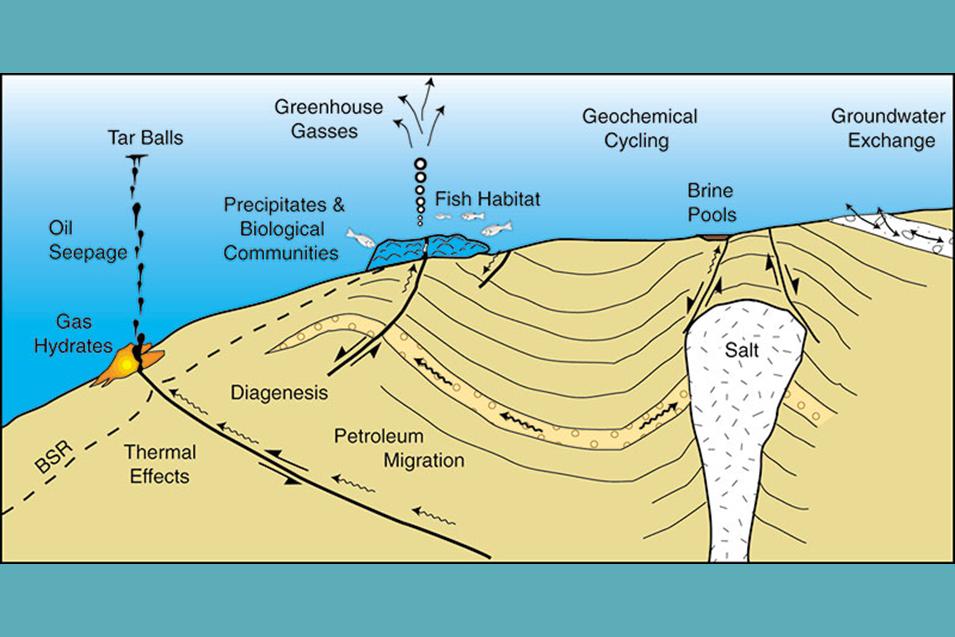
FOSSIL FUELS MELTING ANTARCTICA
Posted on: March 22, 2020
[LINK TO THE HOME PAGE OF THIS SITE]
[RELATED POST ON ANTARCTICA AND SEA LEVEL RISE]
THIS POST IS A CRITICAL REVIEW OF THE CLIMATE CHANGE RESEARCH PAPER {History, mass loss, structure, and dynamic behavior of the Antarctic Ice Sheet, Robin E. Bell1,*, Helene Seroussi2 See all authors and affiliations Science 20 Mar 2020: Vol. 367, Issue 6484, pp. 1321-1325 DOI: 10.1126/science.aaz5489} ABSTRACT (abbreviated) {Satellite measurements show that several regions of Antarctica where ice is exposed to warm ocean waters are losing mass, flowing faster, and retreating. Antarctica’s contribution to sea level rise since 1992 is now 8 millimeters. A continuation of warming ocean waters and increased surface meltwater will trigger faster ice flow, and sea level rise will accelerate.


ABOUT ROBIN ELIZABETH BELL


The lead author of the paper is Professor Robin Bell, Earth Science Professor at Columbia University. Her research emphasis has been Antarctica ice melt and sea level rise with a focus on ice shelves [LINK] . She says that she studies “evidence for changing ice” and that her wake-up call came when the Larsen B ice shelf collapsed in 2002 because “The Antarctic Peninsula is where global temperatures have risen the most, more than 7°F in 50 years“. The focus of her work is catastrophic sea level rise by way of AGW driven ice melt in Antarctica. This unique career may have been the result of her emotional reaction to the spectacle of the Larsen B ice shelf collapse. She has written about this event profusely and described the event as an AGW horror and a product of fossil fuel emissions.
CLAIM=WHAT THE PAPER SAYS. RESPONSE=CRITICAL EVALUATION OF THE CLAIM
CLAIM: GRACE data show mass loss in West Antarctica, focused in the Amundsen and Bellingshausen Sea sectors, and mass gain in some regions of East Antarctica and along Kamb Ice Stream. RESPONSE: This well known pattern of ice melt in Antarctica is described in a related post [LINK] where the difference is interpreted in terms of rocky support for East Antarctic Ice versus oceanic bottoms of West Antarctic glaciers and in terms of geological activity in West Antarctica with the West Antarctic Rift system and the Marie Byrd Mantle Plume cited as the basis for that assessment.
CLAIM: Lowering of the surface elevation has been measured over the 25-year altimetry period and it is pronounced in the Amundsen and Bellingshausen Sea sectors of West Antarctica and Wilkes Land in East Antarctica. Pine Island, Thwaites, and Smith-Pope-Kohler Glaciers experienced the greatest elevation drop over this period, with changes of up to 9 m/year. Mass gain in East Antarctica with rising elevation is attributed to increased snowfall. RESPONSE: The pattern of surface ice loss is consistent with its geological interpretation described in the related post cited above [LINK] and inconsistent with a uniform atmospheric cause thought to be driven by the rising greenhouse effect of fossil fuel emissions such that the ice loss in Antarctica and its sea level effects can be attenuated with climate action in the form of reducing fossil fuel emissions.
CLAIM: Velocity measurements show that changes in ice sheet velocity are striking in the Peninsula, where a substantial acceleration of glaciers feeding the Larsen ice shelves was observed after their collapse, as well as in the Amundsen Sea sector. In this region, Pine Island Glacier’s velocity doubled from the 1990s to the 2010s while its grounding line retreated by more than 30 km. The velocity observations are used to calculate the flux of ice discharge into the ocean. RESPONSE: The Antarctic Peninsula and the Pine Island Glacier are both subject to intense geological activity and geothermal heat. That the acceleration is found to be localized to these geothermal hot spots does not imply a uniform atmospheric cause by way of fossil fuel emissions that can be attenuated by reducing fossil fuel emissions.
CLAIM: Between 1950 and 2000, the average air temperature in the Peninsula increased by 4°C. During this warming period, the Larsen A and B ice shelves collapsed in 1995 and 2002, respectively. The glaciers feeding the Larsen B Ice Shelf sped up after the loss of the backward stress or buttressing. Before the Larsen B collapse, the ice shelf surface was covered by lakes, indicating that warming air temperatures and surface meltwater can destabilize ice shelves, leading to faster flow of Antarctic ice into the global oceans and highlighting the protecting role of ice shelves. RESPONSE: Monthly mean mid troposphere temperatures from October 1994 to April 2002 for South Polar land and ocean surfaces are shown in the chart below. No significant warming is seen that would explain meltwater lakes on the top of the ice shelves either in 1995 or in 2002. Therefore, the localized warming trend found only on the Antarctic Peninsula in the period 1950-2000 does not have an AGW climate change interpretation such that it can be attributed to fossil fuel emissions and that it could have been prevented with climate action in the form of reducing emissions. This tiny corner of Antarctica is known to be extremely geologically active by way of the West Antarctic Rift system below it and is also known for the prevalence of katabatic (foehn) winds that can create melt ponds on ice shelves as seen in the bibliography below . The more likely cause of this localized warming event and ice shelf collapse is therefore a localized warming phenomenon such as geothermal heat and katabatic winds both of which are found in the Antarctic Peninsula and neither of which has an AGW climate change interpretation.

GEOTHERMAL HEAT CURIE DEPTH IN ANTARCTICA

CLAIM: These remote sensing observations allow scientists to observe ice sheet changes and decipher the causes of such changes. Both the ocean surrounding Antarctica and the atmosphere, especially in the Peninsula region, have warmed over the 25-year observational record of ice change. Antarctica is losing most of its mass through increased ice flow of the outlet glaciers and ice streams. This contrasts with the Greenland Ice Sheet, where half of the loss is due to faster ice flow and half is due to increased melting of the ice sheet surface (35). Surface melt is not yet a major contributor to ice loss in Antarctica, and global climate models suggest that an increase in snowfall in East Antarctica could partially offset the dynamic mass loss (36). Although these changes have been ongoing for the past three decades, more rapid and dramatic mass loss cannot be excluded. The marine portions of the ice sheet with subglacial topography that deepens inland and glaciers with thick marine terminating fronts are prone to instabilities (37, 38). RESPONSE: Remote sensing observations do allow scientists to observe ice sheet changes but they do not contain information that the cause of those changes is global warming particularly so when these changes are highly localized anomalies in a tiny corner of Antarctica known for high geothermal heat flux as shown in the image above. These observations tell us only that Antarctica is losing ice. They do not tell us that the ice loss is driven by fossil fuel emissions and that they can be attenuated by reducing fossil fuel emissions.
CLAIM: Although the surface waters surrounding Antarctica are cold, the underlying waters of the Circumpolar Deep Water are warmer and can influence the ice sheet when they reach the ice shelves and grounding lines, where the ice becomes afloat. The concentration of changes in West Antarctica points to the dominant role the warming ocean plays in recently observed change (39, 40). RESPONSE: With regard to the anomalous warmth of the Circumpolar Deep Water Circulation (CDWC), it is noted that in a highly geologically active area such as West Antarctica and the Antarctic Ocean in general, a role for geothermal heat cannot be ignored. Recent research papers on the CDWC have pointed to significant geothermal heat sources on the sea floor that offer a more ready explanation for the warmth of the CDWC as can be seen in the papers cited in the bibliography below. The geological activity In West Antarctica and the Antarctic Ocean are described in a related post [LINK] where we see the important role of the West Antarctic Rift system and the Marie Byrd Mantle Plume in the interpretation ocean temperature and ice melt in this region. The relative warmth of the CDWC is not evidence of a “warming ocean” in terms of AGW climate change. The CDWC is warmer than surface water but that warmth does not contain a long term warming trend.

RELEVANT BIBLIOGRAPHY
- Bouzette, Ariane, and Roland Souchez. “Katabatic wind influence on meltwater supply to fuel glacier–substrate interactions at the grounding line, Terra Nova Bay, East Antarctica.” Annals of glaciology 28 (1999): 272-276. The co-isotopic composition, both in δDand in δ 18O, of interbedded debris-rich and clear ice layers, thought to have been formed at the grounding line of Hells Gate Ice Shelf, indicates freezing by a double-diffusion effect between continental meltwater and sea water within a subglacial sediment. A source of meltwater is required to sustain the process, since the temperature of the bed is below the freshwater melting point. The most likely source is a surficially frozen meltwater lake. Rock outcrops, kept mostly snow-free by the action of katabatic winds, absorb solar radiation so local production of liquid water becomes possible in an area with year-round subfreezing air-temperature conditions. The meltwater accumulated in a marginal lake can eventually reach the subglacial substratum near a pinning point where the ice is relatively thin and fractured.
- G. L. Lyon &W. F. Giggenbach, Geothermal activity in Victoria Land, Antarctica. Pages 511-521 | Received 23 Oct 1973, Published online: 07 Jan 2012. Fumarolic ice towers and areas of steaming ground are the only surface manifestations of geothermal activity near the summits of Mounts Melbourne and Erebus, Victoria Land, Antarctica. The distribution, nature, and limited range of the geothermal features reflect the lack of liquid water in the normal environment of these volcanoes, where modes of heat transport are confined to conduction and convection of air and water vapour. Under such conditions, only localised occurrence of liquid water is considered possible.
- Fountain, Andrew G., et al. “Evolution of cryoconite holes and their contribution to meltwater runoff from glaciers in the McMurdo Dry Valleys, Antarctica.” Journal of Glaciology 50.168 (2004): 35-45. Cryoconite holes are water-filled holes in the surface of a glacier caused by enhanced ice melt around trapped sediment. Measurements on the ablation zones of four glaciers in Taylor Valley, Antarctica, show that cryoconite holes cover about 4–6% of the ice surface. They typically vary in diameter from 5 to 145 cm, with depths ranging from 4 to 56 cm. In some cases, huge holes form with 5 m depths and 30 m diameters. Unlike cryoconite holes elsewhere, these have ice lids up to 36 cm thick and melt from within each spring. About one-half of the holes are connected to the near-surface hydrologic system and the remainder are isolated. The duration of isolation, estimated from the chloride accumulation in hole waters, commonly shows ages of several years, with one hole of 10 years. The cryoconite holes in the McMurdo Dry Valleys create a near-surface hydrologic system tens of cm below the ice surface. The glacier surface itself is generally frozen and dry. Comparison of water levels between holes a few meters apart shows independent cycles of water storage and release. Most likely, local freeze–thaw effects control water passage and therefore temporary storage. Rough calculations indicate that the holes generate at least 13% of the observed runoff on the one glacier measured. This hydrologic system represents the transition between a melting ice cover with supraglacial streams and one entirely frozen and absent of water.
- Banwell, Alison F., Douglas R. MacAyeal, and Olga V. Sergienko. “Breakup of the Larsen B Ice Shelf triggered by chain reaction drainage of supraglacial lakes.” Geophysical Research Letters 40.22 (2013): 5872-5876. The explosive disintegration of the Larsen B Ice Shelf poses two unresolved questions: What process (1) set a horizontal fracture spacing sufficiently small to predispose the subsequent ice shelf fragments to capsize and (2) synchronized the widespread drainage of >2750 supraglacial meltwater lakes observed in the days prior to break up? We answer both questions through analysis of the ice shelf’s elastic flexure response to the supraglacial lakes on the ice shelf prior to break up. By expanding the previously articulated role of lakes beyond mere water reservoirs supporting hydrofracture, we show that lake‐induced flexural stresses produce a fracture network with appropriate horizontal spacing to induce capsize‐driven breakup. The analysis of flexural stresses suggests that drainage of a single lake can cause neighboring lakes to drain, which, in turn, causes farther removed lakes to drain. Such self‐stimulating behavior can account for the sudden, widespread appearance of a fracture system capable of driving explosive break up.
- Luckman, Adrian, et al. “Surface melt and ponding on Larsen C Ice Shelf and the impact of föhn winds.” Antarctic Science 26.6 (2014): 625-635. A common precursor to ice shelf disintegration, most notably that of Larsen B Ice Shelf, is unusually intense or prolonged surface melt and the presence of surface standing water. However, there has been little research into detailed patterns of melt on ice shelves or the nature of summer melt ponds. We investigated surface melt on Larsen C Ice Shelf at high resolution using Envisat advanced synthetic aperture radar (ASAR) data and explored melt ponds in a range of satellite images. The improved spatial resolution of SAR over alternative approaches revealed anomalously long melt duration in western inlets. Meteorological modelling explained this pattern by föhn winds which were common in this region. Melt ponds are difficult to detect using optical imagery because cloud-free conditions are rare in this region and ponds quickly freeze over, but can be monitored using SAR in all weather conditions. Melt ponds up to tens of kilometres in length were common in Cabinet Inlet, where melt duration was most prolonged. The pattern of melt explains the previously observed distribution of ice shelf densification, which in parts had reached levels that preceded the collapse of Larsen B Ice Shelf, suggesting a potential role for föhn winds in promoting unstable conditions on ice shelves. [FULL TEXT]
- Fisher, Andrew T., et al. “High geothermal heat flux measured below the West Antarctic Ice Sheet.” Science advances 1.6 (2015): e1500093. The geothermal heat flux is a critical thermal boundary condition that influences the melting, flow, and mass balance of ice sheets, but measurements of this parameter are difficult to make in ice-covered regions. We report the first direct measurement of geothermal heat flux into the base of the West Antarctic Ice Sheet (WAIS), below Subglacial Lake Whillans, determined from the thermal gradient and the thermal conductivity of sediment under the lake. The heat flux at this site is 285 ± 80 mW/m2, significantly higher than the continental and regional averages estimated for this site using regional geophysical and glaciological models. Independent temperature measurements in the ice indicate an upward heat flux through the WAIS of 105 ± 13 mW/m2. The difference between these heat flux values could contribute to basal melting and/or be advected from Subglacial Lake Whillans by flowing water. The high geothermal heat flux may help to explain why ice streams and subglacial lakes are so abundant and dynamic in this region.
- Hubbard, Bryn, et al. “Massive subsurface ice formed by refreezing of ice-shelf melt ponds.” Nature communications 7.1 (2016): 1-6. Surface melt ponds form intermittently on several Antarctic ice shelves. Although implicated in ice-shelf break up, the consequences of such ponding for ice formation and ice-shelf structure have not been evaluated. Here we report the discovery of a massive subsurface ice layer, at least 16 km across, several kilometres long and tens of metres deep, located in an area of intense melting and intermittent ponding on Larsen C Ice Shelf, Antarctica. We combine borehole optical televiewer logging and radar measurements with remote sensing and firn modelling to investigate the layer, found to be ∼10 °C warmer and ∼170 kg m−3 denser than anticipated in the absence of ponding and hitherto used in models of ice-shelf fracture and flow. Surface ponding and ice layers such as the one we report are likely to form on a wider range of Antarctic ice shelves in response to climatic warming in forthcoming decades.
- Lenaerts, J. T. M., et al. “Meltwater produced by wind–albedo interaction stored in an East Antarctic ice shelf.” Nature climate change 7.1 (2017): 58-62. Surface melt and subsequent firn air depletion can ultimately lead to disintegration of Antarctic ice shelves1,2 causing grounded glaciers to accelerate3 and sea level to rise. In the Antarctic Peninsula, foehn winds enhance melting near the grounding line4, which in the recent past has led to the disintegration of the most northerly ice shelves5,6. Here, we provide observational and model evidence that this process also occurs over an East Antarctic ice shelf, where meltwater-induced firn air depletion is found in the grounding zone. Unlike the Antarctic Peninsula, where foehn events originate from episodic interaction of the circumpolar westerlies with the topography, in coastal East Antarctica high temperatures are caused by persistent katabatic winds originating from the ice sheet’s interior. Katabatic winds warm and mix the air as it flows downward and cause widespread snow erosion, explaining >3 K higher near-surface temperatures in summer and surface melt doubling in the grounding zone compared with its surroundings. Additionally, these winds expose blue ice and firn with lower surface albedo, further enhancing melt. The in situ observation of supraglacial flow and englacial storage of meltwater suggests that ice-shelf grounding zones in East Antarctica, like their Antarctic Peninsula counterparts, are vulnerable to hydrofracturing. [FULL TEXT]
- Bell, Robin E., et al. “Antarctic ice shelf potentially stabilized by export of meltwater in surface river.” Nature 544.7650 (2017): 344-348. Meltwater stored in ponds1 and crevasses can weaken and fracture ice shelves, triggering their rapid disintegration2. This ice-shelf collapse results in an increased flux of ice from adjacent glaciers3 and ice streams, thereby raising sea level globally4. However, surface rivers forming on ice shelves could potentially export stored meltwater and prevent its destructive effects. Here we present evidence for persistent active drainage networks—interconnected streams, ponds and rivers—on the Nansen Ice Shelf in Antarctica that export a large fraction of the ice shelf’s meltwater into the ocean. We find that active drainage has exported water off the ice surface through waterfalls and dolines for more than a century. The surface river terminates in a 130-metre-wide waterfall that can export the entire annual surface melt over the course of seven days. During warmer melt seasons, these drainage networks adapt to changing environmental conditions by remaining active for longer and exporting more water. Similar networks are present on the ice shelf in front of Petermann Glacier, Greenland, but other systems, such as on the Larsen C and Amery Ice Shelves, retain surface water at present. The underlying reasons for export versus retention remain unclear. Nonetheless our results suggest that, in a future warming climate, surface rivers could export melt off the large ice shelves surrounding Antarctica—contrary to present Antarctic ice-sheet models1, which assume that meltwater is stored on the ice surface where it triggers ice-shelf disintegration.
- Kingslake, Jonathan, et al. “Widespread movement of meltwater onto and across Antarctic ice shelves.” Nature 544.7650 (2017): 349-352. Surface meltwater drains across ice sheets, forming melt ponds that can trigger ice-shelf collapse1,2, acceleration of grounded ice flow and increased sea-level rise3,4,5. Numerical models of the Antarctic Ice Sheet that incorporate meltwater’s impact on ice shelves, but ignore the movement of water across the ice surface, predict a metre of global sea-level rise this century5 in response to atmospheric warming6. To understand the impact of water moving across the ice surface a broad quantification of surface meltwater and its drainage is needed. Yet, despite extensive research in Greenland7,8,9,10 and observations of individual drainage systems in Antarctica10,11,12,13,14,15,16,17, we have little understanding of Antarctic-wide surface hydrology or how it will evolve. Here we show widespread drainage of meltwater across the surface of the ice sheet through surface streams and ponds (hereafter ‘surface drainage’) as far south as 85° S and as high as 1,300 metres above sea level. Our findings are based on satellite imagery from 1973 onwards and aerial photography from 1947 onwards. Surface drainage has persisted for decades, transporting water up to 120 kilometres from grounded ice onto and across ice shelves, feeding vast melt ponds up to 80 kilometres long. Large-scale surface drainage could deliver water to areas of ice shelves vulnerable to collapse, as melt rates increase this century. While Antarctic surface melt ponds are relatively well documented on some ice shelves, we have discovered that ponds often form part of widespread, large-scale surface drainage systems. In a warming climate, enhanced surface drainage could accelerate future ice-mass loss from Antarctic, potentially via positive feedbacks between the extent of exposed rock, melting and thinning of the ice sheet.
- Mashayek, A., et al. “The role of the geothermal heat flux in driving the abyssal ocean circulation.” Geophysical Research Letters 40.12 (2013): 3144-3149. [FULL TEXT] The results presented in this paper demonstrate that the geothermal heat flux (GHF) from the solid Earth into the ocean plays a non‐negligible role in determining both abyssal stratification and circulation strength. Based upon an ocean data set, we show that the map of upward heat flux at the ocean floor is consistent (within a factor of 2) with the ocean floor age‐dependent map of GHF. The observed buoyancy flux above the ocean floor is consistent with previous suggestions that the GHF acts to erode the abyssal stratification and thereby enhances the strength of the abyssal circulation. Idealized numerical simulations are performed using a zonally averaged single‐basin model which enables us to address the GHF impact as a function of the depth dependence of diapycnal diffusivity. We show that ignoring this vertical variation leads to an under‐prediction of the influence of the GHF on the abyssal circulation. Independent of the diffusivity profile, introduction of the GHF in the model leads to steepening of the Southern Ocean isopycnals and to strengthening of the eddy‐induced circulation and the Antarctic bottom water cell. The enhanced circulation ventilates the GHF derived heating to shallow depths, primarily in the Southern Ocean.
- Downes, Stephanie M., et al. [LINK] “The transient response of southern ocean circulation to geothermal heating in a global climate model.” Journal of Climate 29.16 (2016): 5689-5708. Model and observational studies have concluded that geothermal heating significantly alters the global overturning circulation and the properties of the widely distributed Antarctic Bottom Water. Here two distinct geothermal heat flux datasets are tested under different experimental designs in a fully coupled model that mimics the control run of a typical Coupled Model Intercomparison Project (CMIP) climate model. The regional analysis herein reveals that bottom temperature and transport changes, due to the inclusion of geothermal heating, are propagated throughout the water column, most prominently in the Southern Ocean, with the background density structure and major circulation pathways acting as drivers of these changes. While geothermal heating enhances Southern Ocean abyssal overturning circulation by 20%–50%, upwelling of warmer deep waters and cooling of upper ocean waters within the Antarctic Circumpolar Current (ACC) region decrease its transport by 3–5 Sv (1 Sv = 106 m3 s−1). The transient responses in regional bottom temperature increases exceed 0.1°C. The large-scale features that are shown to transport anomalies far from their geothermal source all exist in the Southern Ocean. Such features include steeply sloping isopycnals, weak abyssal stratification, voluminous southward flowing deep waters and exported bottom waters, the ACC, and the polar gyres. Recently the Southern Ocean has been identified as a prime region for deep ocean warming; geothermal heating should be included in climate models to ensure accurate representation of these abyssal temperature changes.
- Barnes, Jowan M., et al. “Idealised modelling of ocean circulation driven by conductive and hydrothermal fluxes at the seabed.” Ocean Modelling 122 (2018): 26-35. [FULL TEXT] Geothermal heating is increasingly recognised as an important factor affecting ocean circulation, with modelling studies suggesting that this heat source could lead to first-order changes in the formation rate of Antarctic Bottom Water, as well as a significant warming effect in the abyssal ocean. Where it has been represented in numerical models, however, the geothermal heat flux into the ocean is generally treated as an entirely conductive flux, despite an estimated one third of the global geothermal flux being introduced to the ocean via hydrothermal sources. A modelling study is presented which investigates the sensitivity of the geothermally forced circulation to the way heat is supplied to the abyssal ocean. An analytical two-dimensional model of the circulation is described, which demonstrates the effects of a volume flux through the ocean bed. A simulation using the NEMO numerical general circulation model in an idealised domain is then used to partition a heat flux between conductive and hydrothermal sources and explicitly test the sensitivity of the circulation to the formulation of the abyssal heat flux. Our simulations suggest that representing the hydrothermal flux as a mass exchange indeed changes the heat distribution in the abyssal ocean, increasing the advective heat transport from the abyss by up to 35% compared to conductive heat sources. Consequently, we suggest that the inclusion of hydrothermal fluxes can be an important addition to course-resolution ocean models.
- Downes, Stephanie M., et al. “Hydrothermal heat enhances abyssal mixing in the Antarctic Circumpolar Current.” Geophysical Research Letters 46.2 (2019): 812-821. [LINK] Upwelling in the world’s strongest current, the Antarctic Circumpolar Current, is thought to be driven by wind stress, surface buoyancy flux, and mixing generated from the interaction between bottom currents and rough topography. However, the impact of localized injection of heat by hydrothermal vents where the Antarctic Circumpolar Current interacts with mid‐ocean ridges remains poorly understood. Here a circumpolar compilation of helium and physical measurements are used to show that while geothermal heat is transferred to the ocean over a broad area by conduction, heat transfer by convection dominates near hydrothermal vents. Buoyant hydrothermal plumes decrease stratification above the vent source and increase stratification to the south, altering the local vertical diffusivity and diapycnal upwelling within 500 m of the sea floor by an order of magnitude. Both the helium tracer and stratification signals induced by hydrothermal input are advected by the flow and influence properties downstream.
AN ATMOSPHERE BIAS: PART-2
Posted on: March 20, 2020


THE PETM THERMAL MAXIMUM
[LINK TO THE HOME PAGE OF THIS SITE]
THIS POST IS A CRITICAL REVIEW OF THREE PUBLICATIONS THAT ATTEMPT THE ATTRIBUTION OF THE GLOBAL WARMING EVENT OF THE PALEOCENE EOCENE THERMAL MAXIMUM (PETM) TO THE GREENHOUSE EFFECT OF ATMOSPHERIC CARBON DIOXIDE.
THE ESSENCE OF THE ARGUMENT IS THE ILLOGIC THAT THE EXTREME HEAT DEEP IN THE OCEAN THAT HAD DRIVEN THE CARBON DIOXIDE FROM THE OCEAN TO THE ATMOSPHERE WAS THE CREATION OF THE GREENHOUSE EFFECT OF CO2 ONCE IT DID GET INTO THE ATMOSPHERE.
THIS ARGUMENT IS THEN USED TO SUPPORT THE PROPOSITION THAT THE PETM SHOULD SERVE AS A CAUTIONARY TALE FOR WHAT IS TO COME IN AGW CLIMATE CHANGE OF THE INDUSTRIAL ECONOMY IF WE DO NOT TAKE TIMELY CLIMATE ACTION. [LINK]
RELATED POST: CAN THE OCEAN ACIDIFIY ITSELF: [LINK]
- A brief overview of the PETM event is presented in a related post along with a relevant bibliography [LINK] where we find that there was a 10,000 year (or so) period of global warming about 55 to 56 million years ago. The warming is found in the atmosphere, in sea surface temperature, and in the deep ocean. Temperatures in the deep ocean rose by 4C from 11C to 15C while SST warmed by 8 to 10C with SST as high as 33C in the mid-latitudes and 23C in the Arctic. Global mean surface temperatures rose by 5 to 9C.
- In paleo terminology, these changes are described as “abrupt” but it should be noted that a warming of 10C took place over a period of 10,000 years corresponds to a warming rate of 0.1C per century. The paleo data also show that over the same period of time Carbon13 levels in both oceans and atmosphere fell by 0.2% to 0.4% from the norm. It is significant that this carbon isotope excursion is found in both atmosphere and ocean. The excursion implies that carbon in the current carbon cycle had been combined with geological carbon that had yet not been exposed to the atmosphere.
- Oceanic oxygen depletion: Warming of deep waters was followed by oxygen deficiency in the deep ocean as seen in the extinction of 30–50% of the oceans bottom dwelling species. Oxygen depletion implies that warming was associated with oxidation of some kind.
- Ocean Acidification: Coincident with oceanic oxygen depletion, there was a rapid decline in pH down to depths greater than 3km of the ocean. The data indicate a very large global oxidation event in the ocean that generated large quantities of carbon dioxide.
- Increase in Atmospheric Carbon Dioxide: Atmospheric CO2 levels show a large uncertainty range from 230 to 630 ppm that is thought to have increased by more than 70% in course of the 10,000-year PETM event.
- The attempt to describe the observed warming of the PETM in terms of the greenhouse effect of atmospheric CO2 and thereby to draw theoretical parallels with the current warming episode has not yielded useful results because it yields gross anomalies in terms of climate sensitivity and also because some of the warming events recorded came before the increase in atmospheric CO2. However, as we show below, a strong interest persists such that research efforts continue to find ways to describe the PETM warming, ocean heat content, and ocean acidification in terms of the steep rise in atmospheric CO2 concentration found in the paleo data.
- A question that does not have a direct and explicit answer in the paleo data is what had caused the large deep-ocean oxidation event that warmed the ocean, depleted its oxygen, increased its inorganic carbon concentration, and injected carbon dioxide into the atmosphere. The possibilities that have been explored are methane hydrates in ocean sediments that were dissociated into methane by a deep ocean heat source, likely to be geothermal, that was hot enough not just to break down the hydrate and produce methane but also to ignite and oxidize the methane to water and carbon dioxide. This explains the ocean’s oxygen depletion.
- An alternative theory identifies the mantle as a direct source of both carbon and heat (Svenson 2004). Since the Svenson paper, it is not almost universally conceded that the intermediate role for methane hydrates is unnecessary. In recent papers we find that the overall consensus of researchers in this field, including principal investigators James Zachos, Philip Gingerich, and others now favor the Svenson theory that the mantle was the direct cause of the PETM event without the an intermediate role for methane hydrates previously assumed. Thus the current state of the PETM theory is that it was an entirely geological event.
- However, the issue of great interest in the PETM in the era of AGW climate change warming since the end of the LIA, described as a creation of fossil fuel emissions of the industrial economy, is the role of the greenhouse effect of atmospheric carbon dioxide in the PETM and its various horrific events including global warming, ocean heat content, ocean acidification, and mass extinctions of ocean flora and fauna ultimately driven by rising atmospheric CO2 concentration. Here we present three such papers and their critical evaluation.
- REFERENCE ARTICLE#1: SUDDEN ANCIENT GLOBAL WARMING EVENT TRACED TO MAGMA FLOOD [LINK] . This article from Quanta magazine was published March 19, 2020. The author is “contributing writer” Howard Lee. It cites James Zachos, Lee Kemp, Appy Sluijs, and Stephen Jones and a recent paper by Jones to conclude that the PETM was a purely igneous geological event with warming and carbon release from the ocean attributed directly to magma from the mantle without the intermediate role of methane hydrates. It concludes that the PETM was indeed a purely geological event. Unlike media articles on the subject, it makes no effort to relate the PETM to AGW or to relate the horrific ocean warming, ocean acidification, and mass extinction of ocean flora and fauna to atmospheric CO2. It admits that the rise in atmospheric CO2 of 70% was not the cause of the PETM but an effect of the PETM in terms of its geological cause.
- REFERENCE ARTICLE#2: NEW RESEARCH REVEALS PETM CLIMATE WARMING WAS GEOLOGICALLY INSTANTANEOUS [LINK] , This article in Planet Watch magazine was written by Andrew Burger in October 2013. It says that the PETM event released 3,000 gigatons of carbon into the atmosphere from hydrocarbon-rich organic mud-stone, and methane hydrate deposits on the seafloor of the continental shelves. And that the 70% rise in atmospheric CO2 thus caused in turn caused rapid global warming as well as ocean acidification, steep rise in ocean heat content, and mass extinctions in the ocean.
- It is often overlooked that the mass extinction of the PETM event was purely oceanic. In fact that this mass extinction is credited with the creation of new species, in particular, the modern land mammal from which we are derived. Without the PETM there would not have been humans. Mass extinctions are natural and not an evil that is extraneous to nature such that it is the job of human ecologists to prevent mass extinctions.In addition to forcing rapid warming, this led to an abrupt rise in the acidity of the oceans, which, in turn, led to mass extinctions of the phytoplankton that not only form the base of the marine food chain, but produce as much as half the oxygen in the atmosphere and absorb as much as half the total atmospheric CO2 sequestered as part of the carbon cycle. Similarly drastic changes have been found in terrestrial flora and fauna.
- The urge to explain the PETM event in terms of the greenhouse effect of atmospheric CO2 thus serves as an example of the atmosphere bias in AGW climate science that leads to these kinds of extreme interpretations of the PETM geological event such that a rise in atmospheric CO2 caused by geological events in the ocean is inverted and atmospheric CO2 is then interpreted as the the cause of the oceanic events by way of the greenhouse effect of carbon dioxide.
- REFERENCE ARTICLE#3: Caldeira Lab Research:Paleoclimate and geochemical cycles. An Ancient Carbon Mystery: Here the authors use the PETM to forecast how the current AGW warming will evolve in the future by studying the greenhouse effect of CO2 in the PETM and with the assumption that the PETM was the creation of rising CO2. It says that “the Paleocene-Eocene Thermal Maximum (PETM)—may be the best ancient analog for future increases in atmospheric CO2. But how well do we understand this event?”. By thus drawing an analogy betweenn AGW climate change and the PETM, the authors claim that they can use the PETM to understand how AGW will evolve in the future.
- Specifically, they use the PETM to understand climate sensitivity, as seen in the image below. Here, for various estimates of how much carbon was driven from the ocean to the atmosphere they estimate what the climate sensitivity had to be to cause the ocean to drive that much carbon into the atmosphere. We propose here that this causation reasoning is invalid because it uses circular reasoning. That The atmosphere caused the ocean to warm because ocean warming caused atmospheric carbon dioxide to rise contains two hypotheses that cancel each other out in the sense that they can’t both be true. Such publications of climate science reveal a deep seated atmosphere bias that contains a predisposition to the idea that the greenhouse gas effect of atmospheric CO2 drives climate and this predisposition limits the ability of climate science to see climate data in the broader context that includes the role of earth’s geological forces in climate phenomena as described in related posts [LINK] [LINK] [LINK] [LINK]

CONCLUSION
The proposed heat trapping effect of atmospheric CO2 could not have initiated the PETM warming because the oceanic carbon enrichment and oxidation events preceded the rise in atmospheric CO2; and the rise in atmospheric CO2 is poorly quantified. Also, using the IPCC climate sensitivity range of ECS = [1.5, 4.5] in conjunction with the best guess for the rise in atmospheric CO2 concentration does not explain the amount of surface warming. It is therefore possible that other sources of heat, possibly geothermal, may have been what injected large quantities of geological carbon into the ocean, oxidized the carbon, depleted the ocean’s oxygen, heated the ocean, reduced ocean pH, and released the oxidation CO2 into the atmosphere causing atmospheric CO2 to rise. The motivation to reverse this causation sequence and explain the PETM in terms of the greenhouse effect of atmospheric CO2 that was created by the event, is explained in terms of an atmosphere bias in climate science that prevents climate scientists from consideration of geological forces of the planet that are relevant to the oceanic and surface phenomena under study.
FOOTNOTES
FOOTNOTE#1: It should be mentioned in this context that the failed obsession of climate science with the collapse of the West Antarctic ice sheet causing catastrophic sea level rise; and the horror of the acidification of the ocean with fossil fuel emissions that have been repeatedly used to justify their proposed costly climate action plans are derived from previous realities from the paleo record that cannot be related to the current warming trend of the Holocene. In the previous interglacial, the Eemian, the WAIS had collapsed with catastrophic sea level rise of 5 to 9 meters. This had happened at the onset of the interglacial in the first millennium of the Eemian and its attempted recreation 10,000 years into the Holocene has been a comical failure. Similarly, the ocean acidification fear was borrowed from the PETM, the gross mismatch between the PETM and the Holocene notwithstanding such that its failure can be understood in that light.
FOOTNOTE #2: The most dramatic change and the one most relevant to humans is that the PETM is credited with the rapid expansion of mammals on land and the first appearance of the modern orders of mammals from which we are derived. For details please see the various works of Paleontologist Philip Dean Gingerich. Mass extinction is the way nature works. It is not something that requires humans to take control of nature and ensure that mass extinctions are not allowed to happen. Humans are part of nature and mass extinctions is how nature works. The great interest of humans in managing nature is unnatural and illogical.
BIBLIOGRAPHY
- 1995: Dickens, Gerald R., et al. “Dissociation of oceanic methane hydrate as a cause of the carbon isotope excursion at the end of the Paleocene.” Paleoceanography and Paleoclimatology10.6 (1995): 965-971. Isotopic records across the “Latest Paleocene Thermal Maximum“ (LPTM) indicate that bottom water temperature increased by more than 4°C during a brief time interval (<104years) of the latest Paleocene (∼55.6 Ma). There also was a coeval −2 to −3‰ excursion in the δ13C of the ocean/atmosphere inorganic carbon reservoir. Given the large mass of this reservoir, a rapid δ13C shift of this magnitude is difficult to explain within the context of conventional hypotheses for changing the mean carbon isotope composition of the ocean and atmosphere. However, a direct consequence of warming bottom water temperature from 11 to 15°C over 104 years would be a significant change in sediment thermal gradients and dissociation of oceanic CH4 hydrate at locations with intermediate water depths. In terms of the present‐day oceanic CH4 hydrate reservoir, thermal dissociation of oceanic CH4 hydrate during the LPTM could have released greater than 1.1 to 2.1 × 10¹⁸ g of carbon with a δ13C of approximately −60‰. The release and subsequent oxidation of this amount of carbon is sufficient to explain a −2 to −3‰ excursion in δ13C across the LPTM. Fate of CH4 in oceanic hydrates must be considered in developing models of the climatic and paleoceanographic regimes that operated during the LPTM.
- 1997: Dickens, Gerald R., Maria M. Castillo, and James CG Walker. “A blast of gas in the latest Paleocene: Simulating first-order effects of massive dissociation of oceanic methane hydrate.” Geology 25.3 (1997): 259-262. Carbonate and organic matter deposited during the latest Paleocene thermal maximum is characterized by a remarkable −2.5‰ excursion in δ13C that occurred over ∼104 yr and returned to near initial values in an exponential pattern over ∼2 × 10⁵ yr. It has been hypothesized that this excursion signifies transfer of 1.4 to 2.8 × 10¹⁸ g of CH4 from oceanic hydrates to the combined ocean-atmosphere inorganic carbon reservoir. A scenario with 1.12 × 10¹⁸ g of CH4 is numerically simulated here within the framework of the present-day global carbon cycle to test the plausibility of the hypothesis. We find that (1) the δ13C of the deep ocean, shallow ocean, and atmosphere decreases by −2.3‰ over 104 yr and returns to initial values in an exponential pattern over ∼2 × 10⁵ yr; (2) the depth of the lysocline shoals by up to 400 m over 104 yr, and this rise is most pronounced in one ocean region; and (3) global surface temperature increases by ∼2 °C over 104 yr and returns to initial values over ∼2 × 10⁶ yr. The first effect is quantitatively consistent with the geologic record; the latter two effects are qualitatively consistent with observations. Thus, significant CH4 release from oceanic hydrates is a plausible explanation for observed carbon cycle perturbations during the thermal maximum. This conclusion is of broad interest because the flux of CH4 invoked during the maximum is of similar magnitude to that released to the atmosphere from present-day anthropogenic CH4 sources.
- 2002: Thomas, Deborah J., et al. “Warming the fuel for the fire: Evidence for the thermal dissociation of methane hydrate during the Paleocene-Eocene thermal maximum.” Geology30.12 (2002): 1067-1070. Dramatic warming and upheaval of the carbon system at the end of the Paleocene Epoch have been linked to massive dissociation of sedimentary methane hydrate. However, testing the Paleocene-Eocene thermal maximum hydrate dissociation hypothesis has been hindered by the inability of available proxy records to resolve the initial sequence of events. The cause of the Paleocene-Eocene thermal maximum carbon isotope excursion remains speculative, primarily due to uncertainties in the timing and duration of the Paleocene-Eocene thermal maximum. We present new high-resolution stable isotope records based on analyses of single planktonic and benthic foraminiferal shells from Ocean Drilling Program Site 690 (Weddell Sea, Southern Ocean), demonstrating that the initial carbon isotope excursion was geologically instantaneous and was preceded by a brief period of gradual surface-water warming. Both of these findings support the thermal dissociation of methane hydrate as the cause of the Paleocene-Eocene thermal maximum carbon isotope excursion. Furthermore, the data reveal that the methane-derived carbon was mixed from the surface ocean downward, suggesting that a significant fraction of the initial dissociated hydrate methane reached the atmosphere prior to oxidation.
- 2001: Katz, Miriam, et al. Uncorking the bottle: What triggered the Paleocene/Eocene thermal maximum methane release? Paleoceanography 16.6 (2001): 549-562. The Paleocene/Eocene thermal maximum (PETM) was a time of rapid global warming in both marine and continental realms that has been attributed to a massive methane (CH4) release from marine gas hydrate reservoirs. Previously proposed mechanisms for this methane release rely on a change in deepwater source region(s) to increase water temperatures rapidly enough to trigger the massive thermal dissociation of gas hydrate reservoirs beneath the seafloor. To establish constraints on thermal dissociation, we model heat flow through the sediment column and show the effect of the temperature change on the gas hydrate stability zone through time. In addition, we provide seismic evidence tied to borehole data for methane release along portions of the U.S. continental slope; the release sites are proximal to a buried Mesozoic reef front. Our model results, release site locations, published isotopic records, and ocean circulation models neither confirm nor refute thermal dissociation as the trigger for the PETM methane release. In the absence of definitive evidence to confirm thermal dissociation, we investigate an alternative hypothesis in which continental slope failure resulted in a catastrophic methane release. Seismic and isotopic evidence indicates that Antarctic source deepwater circulation and seafloor erosion caused slope retreat along the western margins of the North Atlantic in the late Paleocene. Continued erosion or seismic activity along the oversteepened continental margin may have allowed methane to escape from gas reservoirs trapped between the frozen hydrate‐bearing sediments and the underlying buried Mesozoic reef front, precipitating the Paleocene/Eocene boundary methane release. An important implication of this scenario is that the methane release caused (rather than resulted from) the transient temperature increase of the PETM. Neither thermal dissociation nor mechanical disruption of sediments can be identified unequivocally as the triggering mechanism for methane release with existing data. Further documentation with high‐resolution benthic foraminiferal isotopic records and with seismic profiles tied to borehole data is needed to clarify whether erosion, thermal dissociation, or a combination of these two was the triggering mechanism for the PETM methane release.
- 2002: Bralower, Timothy J. “Evidence of surface water oligotrophy during the Paleocene‐Eocene thermal maximum: Nannofossil assemblage data from Ocean Drilling Program Site 690, Maud Rise, Weddell Sea.” Paleoceanography 17.2 (2002): 13-1. Nannoplankton assemblages at Ocean Drilling Program Site 690 (Maud Rise, Weddell Sea) experienced an abrupt and dramatic transformation at the onset of the Paleocene‐Eocene Thermal Maximum (PETM) at ∼55 m.y. The major assemblage shift suggests a change from colder, more productive surface waters to warmer, more oligotrophic conditions. Significant restructuring of assemblages during the later part of the PETM indicates that nannoplankton communities were not stable and that surface water conditions changed, although they remained warm and oligotrophic. Combined with benthic foraminiferal assemblage data, nannoplankton assemblage results suggest increased sequestration of nutrients in shelf environments and starvation of the open ocean. Although the PETM was a short‐lived event, it appears to have had long‐term effects on nannoplankton, leading to the extinction of Fasciculithus, a dominant Paleocene genus. The Cretaceous and early Paleogene was a time of remarkable transformation of marine communities [e.g., Vermeij, 1977]. Some of the most dramatic evolutionary changes took place in the protistans. Groups such as the diatoms and planktic foraminifera became fundamental parts of marine food chains during this time. Other groups such as the calcareous nannoplankton and radiolarians underwent wholesale changes in species composition and assemblage structure. The underlying causes of the long‐term evolutionary changes that took place are not well understood [e.g., Roth, 1987; Leckie, 1987; Leckie et al., 2002]. Research over the last decade, however, has established that these groups were also affected by environmental changes that took place over short timescales. In particular, short‐lived (<1 m.y.) global warming events sparked significant biotic turnover in association with dramatic changes in global carbon cycling [e.g., Schlanger et al., 1987; Leckie, 1989; Elder, 1991; Kennett and Stott, 1991; Coccioni et al., 1992; Erba, 1994; Koch et al., 1995; Kelly et al., 1996; Thomas and Shackleton, 1996; Aubry, 1998; Premoli Silva and Sliter, 1999; Premoli Silva et al., 1999]. One of the most extreme and abrupt warming episodes occurred close to the Paleocene/Eocene boundary at ∼55 Ma [Kennett and Stott, 1991; Bralower et al., 1995; Thomas and Shackleton, 1996]. This event, which is known as the Paleocene‐Eocene Thermal Maximum (PETM) [e.g., Zachos et al., 1993], lasted for a period of ∼210 kyr [Norris and Röhl, 1999; Röhl et al., 2000]. The deep and surface oceans warmed by ∼5° and ∼4°–8°C, respectively, during the PETM. The carbon isotopic composition of the ocean and atmosphere decreased by 3–4‰ coeval with the warming event, suggesting a massive perturbation to the global carbon cycle [Kennett and Stott, 1991; Koch et al., 1992; Bains et al., 1999; Norris and Röhl, 1999]. The large magnitude and rate of onset of the carbon isotope excursion (CIE) are most consistent with the sudden dissociation of methane hydrates from continental shelves and slopes [Dickens et al., 1995, 1997; Katz et al., 1999]; CH4 would have immediately contributed to greenhouse warming. The PETM climatic changes affected biota on a global scale, triggering abrupt turnover of benthic and planktic organisms in the ocean [e.g., Kennett and Stott, 1991; Kelly et al., 1996; Speijer and Morsi, 2002], and the rapid radiation of mammals on land [e.g., Gingerich et al., 1980; Maas et al., 1995; Hooker, 1996; Clyde and Gingerich, 1998]. Deep‐sea environmental changes led to an abrupt extinction in benthic foraminiferal communities [e.g., Thomas, 1990; Pak and Miller, 1992; Thomas and Shackleton, 1996; Thomas, 1998]. This benthic foraminiferal extinction (BFE) event [e.g., Tjalsma and Lohmann, 1983] has been well documented in a range of different environments and latitudes [e.g., Kaiho et al., 1996; Speijer et al., 1996]. The response of surface‐dwelling marine organisms to PETM environmental changes appears to have been fundamentally different: tropical planktic foraminifers radiated dramatically during this event [Kelly et al., 1996, 1998]. There have been few high‐resolution investigations of the response of phytoplankton groups such as the calcareous nannoplankton to the PETM. Most previous investigations have considered only long‐term changes in assemblages through the late Paleocene‐early Eocene interval [e.g., Aubry, 1998]. Interpretations of geochemical and biotic investigations disagree as to whether the PETM was characterized by increased or decreased surface water productivity. Tropical plankton at Pacific Site 865 suggests increased oligotrophy [Kelly et al., 1996]; benthic foraminiferal assemblages in open ocean sites also suggest reduced food supply under oligotrophic surface water conditions, whereas assemblages in marginally marine and shelf sites are interpreted as indicating high food supply likely as a result of eutrophic conditions [Thomas and Shackleton, 1996; Speijer and Schmitz, 1998; Thomas, 1998; Thomas et al., 2000]. A widespread bloom of the dinoflagellate Apectodinium in sections deposited in coastal environments is also consistent with high productivity [Crouch et al., 2001]. Bains et al. [2000] interpreted an increase in Ba accumulation rates in the PETM at several open‐ocean sites as evidence for high productivity; these authors concluded that elevated productivity led to increased CO2 draw down, curbing a potential runaway greenhouse. To attempt to resolve the contrast between biotic and geochemical proxies of productivity and to more fully constrain the effects of the PETM on marine phytoplankton, we have carried out a detailed study of calcareous nannofossil assemblages across the PETM at Site 690 (Maud Rise, Weddell Sea; Figure 1). This site contains one of the highest‐quality deep‐sea records of the PETM event. Upper Paleocene sediments are composed of ooze representing nannofossil zone NP9, planktic foraminiferal zones AP4 and AP5, and part of magnetic polarity zone C24r [Aubry et al., 1996]. White to pale brown lithologic cycles caused by oscillations of CaCO3 and clay content appear to correspond to precessional orbital rhythms [Röhl et al., 2000]. These cycles can be used to construct a timescale for Site 690 [Cramer, 2001; D. Thomas, manuscript in preparation, 2002], allowing us to monitor paleoceanographic changes at millennial resolution.
- 2003: Kent, Dennis V., et al. “A case for a comet impact trigger for the Paleocene/Eocene thermal maximum and carbon isotope excursion.” Earth and Planetary Science Letters 211.1-2 (2003): 13-26. We hypothesize that the rapid onset of the carbon isotope excursion (CIE) at the Paleocene/Eocene boundary (∼55 Ma) may have resulted from the accretion of a significant amount of 12C-enriched carbon from the impact of a ∼10 km comet, an event that would also trigger greenhouse warming leading to the Paleocene/Eocene thermal maximum and, possibly, thermal dissociation of seafloor methane hydrate. Indirect evidence of an impact is the unusual abundance of magnetic nanoparticles in kaolinite-rich shelf sediments that closely coincide with the onset and nadir of the CIE at three drill sites on the Atlantic Coastal Plain. After considering various alternative mechanisms that could have produced the magnetic nanoparticle assemblage and by analogy with the reported detection of iron-rich nanophase material at the Cretaceous/Tertiary boundary, we suggest that the CIE occurrence was derived from an impact plume condensate. The sudden increase in kaolinite is thus thought to represent the redeposition on the marine shelf of a rapidly weathered impact ejecta dust blanket. Published reports of a small but significant iridium anomaly at or close to the Paleocene/Eocene boundary provide supportive evidence for an impact.
- 2003: Zachos, James C., et al. “A transient rise in tropical sea surface temperature during the Paleocene-Eocene thermal maximum.” Science 302.5650 (2003): 1551-1554. The Paleocene-Eocene Thermal Maximum (PETM) has been attributed to a rapid rise in greenhouse gas levels. If so, warming should have occurred at all latitudes, although amplified toward the poles. Existing records reveal an increase in high-latitude sea surface temperatures (SSTs) (8° to 10°C) and in bottom water temperatures (4° to 5°C). To date, however, the character of the tropical SST response during this event remains unconstrained. Here we address this deficiency by using paired oxygen isotope and minor element (magnesium/calcium) ratios of planktonic foraminifera from a tropical Pacific core to estimate changes in SST. Using mixed-layer foraminifera, we found that the combined proxies imply a 4° to 5°C rise in Pacific SST during the PETM. These results would necessitate a rise in atmospheric pCO2 to levels three to four times as high as those estimated for the late Paleocene.
- *2004: Svensen, Henrik, et al. “Release of methane from a volcanic basin as a mechanism for initial Eocene global warming.” Nature 429.6991 (2004): 542. A 200,000-yr interval of extreme global warming marked the start of the Eocene epoch about 55 million years ago. Negative carbon- and oxygen-isotope excursions in marine and terrestrial sediments show that this event was linked to a massive and rapid (∼10,000 yr) input of isotopically depleted carbon1,2. It has been suggested previously that extensive melting of gas hydrates buried in marine sediments may represent the carbon source3,4 and has caused the global climate change. Large-scale hydrate melting, however, requires a hitherto unknown triggering mechanism. Here we present evidence for the presence of thousands of hydrothermal vent complexes identified on seismic reflection profiles from the Vøring and Møre basins in the Norwegian Sea. We propose that intrusion of voluminous mantle-derived melts in carbon-rich sedimentary strata in the northeast Atlantic may have caused an explosive release of methane—transported to the ocean or atmosphere through the vent complexes—close to the Palaeocene/Eocene boundary. Similar volcanic and metamorphic processes may explain climate events associated with other large igneous provinces such as the Siberian Traps (∼250 million years ago) and the Karoo Igneous Province (∼183 million years ago).
- 2004: Bowen, Gabriel J., et al. “A humid climate state during the Palaeocene/Eocene thermal maximum.” Nature 432.7016 (2004): 495. An abrupt climate warming of 5 to 10 °C during the Palaeocene/Eocene boundary thermal maximum (PETM) 55 Myr ago is linked to the catastrophic release of ∼1,050–2,100 Gt of carbon from sea-floor methane hydrate reservoirs1. Although atmospheric methane, and the carbon dioxide derived from its oxidation, probably contributed to PETM warming, neither the magnitude nor the timing of the climate change is consistent with direct greenhouse forcing by the carbon derived from methane hydrate. Here we demonstrate significant differences between marine2,3 and terrestrial4,5,6 carbon isotope records spanning the PETM. We use models of key carbon cycle processes7,8,9 to identify the cause of these differences. Our results provide evidence for a previously unrecognized discrete shift in the state of the climate system during the PETM, characterized by large increases in mid-latitude tropospheric humidity and enhanced cycling of carbon through terrestrial ecosystems. A more humid atmosphere helps to explain PETM temperatures, but the ultimate mechanisms underlying the shift remain unknown.
- 2005: Tripati, Aradhna, and Henry Elderfield. “Deep-sea temperature and circulation changes at the Paleocene-Eocene thermal maximum.” Science 308.5730 (2005): 1894-1898. A rapid increase in greenhouse gas levels is thought to have fueled global warming at the Paleocene-Eocene Thermal Maximum (PETM). Foraminiferal magnesium/calcium ratios indicate that bottom waters warmed by 4° to 5°C, similar to tropical and subtropical surface ocean waters, implying no amplification of warming in high-latitude regions of deep-water formation under ice-free conditions. Intermediate waters warmed before the carbon isotope excursion, in association with down-welling in the North Pacific and reduced Southern Ocean convection, supporting changing circulation as the trigger for methane hydrate release. A switch to deep convection in the North Pacific at the PETM onset could have amplified and sustained warming.
- 2005: Zachos, James C., et al. “Rapid acidification of the ocean during the Paleocene-Eocene thermal maximum.” Science308.5728 (2005): 1611-1615. The Paleocene-Eocene thermal maximum (PETM) has been attributed to the rapid release of ∼2000 × 109 metric tons of carbon in the form of methane. In theory, oxidation and ocean absorption of this carbon should have lowered deep-sea pH, thereby triggering a rapid (<10,000-year) shoaling of the calcite compensation depth (CCD), followed by gradual recovery. Here we present geochemical data from five new South Atlantic deep-sea sections that constrain the timing and extent of massive sea-floor carbonate dissolution coincident with the PETM. The sections, from between 2.7 and 4.8 kilometers water depth, are marked by a prominent clay layer, the character of which indicates that the CCD shoaled rapidly (<10,000 years) by more than 2 kilometers and recovered gradually (>100,000 years). These findings indicate that a large mass of carbon (»2000 × 109 metric tons of carbon) dissolved in the ocean at the Paleocene-Eocene boundary and that permanent sequestration of this carbon occurred through silicate weathering feedback.
- 2006: Higgins, John A., and Daniel P. Schrag. “Beyond methane: towards a theory for the Paleocene–Eocene thermal maximum.” Earth and Planetary Science Letters 245.3-4 (2006): 523-537. Extreme global warmth and an abrupt negative carbon isotope excursion during the Paleocene–Eocene Thermal Maximum (PETM) have been attributed to a massive release of methane hydrate from sediments on the continental slope [1]. However, the magnitude of the warming (5 to 6 °C [2],[3]) and rise in the depth of the CCD (> 2 km; [4]) indicate that the size of the carbon addition was larger than can be accounted for by the methane hydrate hypothesis. Additional carbon sources associated with methane hydrate release (e.g. pore-water venting and turbidite oxidation) are also insufficient. We find that the oxidation of at least 5000 Gt C of organic carbon is the most likely explanation for the observed geochemical and climatic changes during the PETM, for which there are several potential mechanisms. Production of thermogenic CH4 and CO2during contact metamorphism associated with the intrusion of a large igneous province into organic rich sediments [5] is capable of supplying large amounts of carbon, but is inconsistent with the lack of extensive carbon loss in metamorphosed sediments, as well as the abrupt onset and termination of carbon release during the PETM. A global conflagration of Paleocene peatlands [6] highlights a large terrestrial carbon source, but massive carbon release by fire seems unlikely as it would require that all peatlands burn at once and then for only 10 to 30 ky. In addition, this hypothesis requires an order of magnitude increase in the amount of carbon stored in peat. The isolation of a large epicontinental seaway by tectonic uplift associated with volcanism or continental collision, followed by desiccation and bacterial respiration of the aerated organic matter is another potential mechanism for the rapid release of large amounts of CO2. In addition to the oxidation of the underlying marine sediments, the desiccation of a major epicontinental seaway would remove a large source of moisture for the continental interior, resulting in the desiccation and bacterial oxidation of adjacent terrestrial wetlands.
- 2006: Zachos, James C., et al. “Extreme warming of mid-latitude coastal ocean during the Paleocene-Eocene Thermal Maximum: Inferences from TEX86 and isotope data.” Geology34.9 (2006): 737-740. Changes in sea surface temperature (SST) during the Paleocene-Eocene Thermal Maximum (PETM) have been estimated primarily from oxygen isotope and Mg/Ca records generated from deep-sea cores. Here we present a record of sea surface temperature change across the Paleocene-Eocene boundary for a nearshore, shallow marine section located on the eastern margin of North America. The SST record, as inferred from TEX86 data, indicates a minimum of 8 °C of warming, with peak temperatures in excess of 33 °C. Similar SSTs are estimated from planktonic foraminifer oxygen isotope records, although the excursion is slightly larger. The slight offset in the oxygen isotope record may reflect on seasonally higher runoff and lower salinity.
- 2006: Sluijs, Appy, et al. “Subtropical Arctic Ocean temperatures during the Palaeocene/Eocene thermal maximum.” Nature441.7093 (2006): 610. The Palaeocene/Eocene thermal maximum, ∼55 million years ago, was a brief period of widespread, extreme climatic warming1,2,3, that was associated with massive atmospheric greenhouse gas input4. Although aspects of the resulting environmental changes are well documented at low latitudes, no data were available to quantify simultaneous changes in the Arctic region. Here we identify the Palaeocene/Eocene thermal maximum in a marine sedimentary sequence obtained during the Arctic Coring Expedition5. We show that sea surface temperatures near the North Pole increased from ∼18 °C to over 23 °C during this event. Such warm values imply the absence of ice and thus exclude the influence of ice-albedo feedbacks on this Arctic warming. At the same time, sea level rose while anoxic and euxinic conditions developed in the ocean’s bottom waters and photic zone, respectively. Increasing temperature and sea level match expectations based on palaeoclimate model simulations6, but the absolute polar temperatures that we derive before, during and after the event are more than 10 °C warmer than those model-predicted. This suggests that higher-than-modern greenhouse gas concentrations must have operated in conjunction with other feedback mechanisms—perhaps polar stratospheric clouds7 or hurricane-induced ocean mixing8—to amplify early Palaeogene polar temperatures.
- 2006: Gingerich, Philip D. “Environment and evolution through the Paleocene–Eocene thermal maximum.” Trends in ecology & evolution 21.5 (2006): 246-253. The modern orders of mammals, Artiodactyla, Perissodactyla and Primates (APP taxa), first appear in the fossil record at the Paleocene–Eocene boundary, c. 55 million years ago. Their appearance on all three northern continents has been linked to diversification and dispersal in response to rapid environmental change at the beginning of a worldwide 100 000–200 000-year Paleocene–Eocene thermal maximum (PETM) and carbon isotope excursion. As I discuss here, global environmental events such as the PETM have had profound effects on evolution in the geological past and must be considered when modeling the history of life. The PETM is also relevant when considering the causes and consequences of global greenhouse warming.
- 2007: Röhl, Ursula, et al. “On the duration of the Paleocene‐Eocene thermal maximum (PETM).” Geochemistry, Geophysics, Geosystems 8.12 (2007). The Paleocene‐Eocene thermal maximum (PETM) is one of the best known examples of a transient climate perturbation, associated with a brief, but intense, interval of global warming and a massive perturbation of the global carbon cycle from injection of isotopically light carbon into the ocean‐atmosphere system. One key to quantifying the mass of carbon released, identifying the source(s), and understanding the ultimate fate of this carbon is to develop high‐resolution age models. Two independent strategies have been employed, cycle stratigraphy and analysis of extraterrestrial helium (HeET), both of which were first tested on Ocean Drilling Program (ODP) Site 690. These two methods are in agreement for the onset of the PETM and initial recovery, or the clay layer (“main body”), but seem to differ in the final recovery phase of the event above the clay layer, where the carbonate contents rise and carbon isotope values return toward background values. Here we present a state‐of‐the‐art age model for the PETM derived from a new orbital chronology developed with cycle stratigraphic records from sites drilled during ODP Leg 208 (Walvis Ridge, Southeastern Atlantic) integrated with published records from Site 690 (Weddell Sea, Southern Ocean, ODP Leg 113). During Leg 208, five Paleocene‐Eocene (P‐E) boundary sections (Sites 1262 to 1267) were recovered in multiple holes over a depth transect of more than 2200 m at the Walvis Ridge, yielding the first stratigraphically complete P‐E deep‐sea sequence with moderate to relatively high sedimentation rates (1 to 3 cm/ka, where “a” is years). A detailed chronology was developed with nondestructive X‐ray fluorescence (XRF) core scanning records on the scale of precession cycles, with a total duration of the PETM now estimated to be ∼170 ka. The revised cycle stratigraphic record confirms original estimates for the duration of the onset and initial recovery but suggests a new duration for the final recovery that is intermediate to the previous estimates by cycle stratigraphy and HeET. The Paleocene Eocene thermal maximum (PETM) is one of the most abrupt and transient climatic events documented in the geologic record [e.g., Zachos et al., 2001, 2005]. This event was associated with pronounced warming of the oceans and atmosphere, changes in ocean chemistry, and reorganization of the global carbon cycle [Kennett and Stott, 1991; Koch et al., 1992; Thomas et al., 2002; Zachos et al., 2003, 2005; Tripati and Elderfield, 2005; Sluijs et al., 2006]. Warming of deep waters and subsequent oxygen deficiency may have been responsible for extinction of 30–50% of deep‐sea benthic foraminiferal species [Thomas and Shackleton, 1996] and planktonic biota were affected by changes in surface water habitats [e.g., Kelly et al., 1996; Bralower et al., 2002; Kelly, 2002; Raffi et al., 2005; Gibbs et al., 2006a, 2006b]; global warming also may have led to a pulse of speciation or migration among mammalian groups [e.g., Koch et al., 1992, Bowen et al., 2001; Gingerich, 2003]. The PETM corresponds to a significant (∼3.5–4.5‰) negative carbon isotope excursion (CIE) recorded in marine and terrestrial sections [e.g., Kennett and Stott, 1991; Koch et al., 1992; Bralower et al., 1997; Zachos et al., 2004, 2005; Schouten et al., 2007]. The source and triggering mechanism of this event are still the focus of much debate [e.g., Lourens et al., 2005; Sluijs et al., 2007; Storey et al., 2007]. An orbital trigger for the PETM and similar (but less severe) events has been suggested [Lourens et al., 2005], but the specific orbital parameter association is still not completely resolved [Westerhold et al., 2007]. Other mechanisms that might explain the abruptness of the CIE include the input of methane into the ocean and atmosphere from the dissociation of methane hydrates in continental margin sediments or from the cracking of coal during rifting of the northern North Atlantic Ocean [Dickens et al., 1995, 1997; Svensen et al., 2004]. Identifying potential triggering mechanisms for the PETM, as well as understanding the relationship between forcing and consequences requires a very precise and high‐resolution chronology. For example, quantifying the climate sensitivity requires robust estimates of the mass of carbon released, and hence the rate of the CIE. Until recently, however, estimates of the absolute age of the onset and the duration of the event were poorly constrained, varying between 54.88 and 55.50 Ma, and 100 and 250 ka, respectively [e.g., Kennett and Stott, 1991; Koch et al., 1992; Aubry et al., 1996; Röhl and Abrams, 2000; Röhl et al., 2000; Farley and Eltgroth, 2003; Giusberti et al., 2007]. By using an astronomically calibrated but floating timescale, the age of the onset (54.93 to 54.98 Ma) and the duration (150 to 220 ka) of the CIE were initially determined at Ocean Drilling Program (ODP) Site 1051 [Norris and Röhl, 1999] then refined using combined records from Sites 690 and 1051 [Röhl et al., 2000]. However, because the onset of the PETM in pelagic sequences is marked by a pronounced dissolution layer or condensed interval and the recovery by a lithologically uniform carbonate‐rich interval, an alternative constant flux age model was developed [Farley and Eltgroth, 2003]. This model is based on the concentrations of extraterrestrial He (3HeET) and the assumption that the flux of this isotope to the Earth remained constant during the PETM. Both age models are in agreement for the duration of the main body of the PETM (70–80 ka for the “core”, the onset, peak, and initial recovery phase (rapid rise in δ13C, but low carbonate; here termed phase 1)), but diverge for the final recovery phase of the CIE (slow rise in δ13C, high carbonate; here termed phase II), with orbital age models producing 140 ka for this interval and He age models 30 ka. Identification of cycles in the Ca (or Fe) records in the recovery interval of the Site 690 section is complicated due to the high and uniform carbonate content of the sediments. A new era in Cenozoic paleoceanography was launched with the recovery of Paleogene sediments in multisite depth transects during Ocean Drilling Program Legs 198 (Shatsky Rise, Pacific Ocean [Bralower et al., 2002; Westerhold and Röhl, 2006]) and 208 (Walvis Ridge, Southeast Atlantic Ocean [Zachos et al., 2004]). These expeditions yielded the first high‐quality, stratigraphically complete sedimentary sequences of the early Paleogene, recovered in offset, multiple‐hole sites. The lithologic and geochemical records generated from these cores exhibit the highly cyclic nature of early Paleogene climate, while also demonstrating that the early Eocene Greenhouse World was punctuated by multiple transient global warming events, or hyperthermals [Thomas et al., 2000; Zachos et al., 2004]. The occurrence of multiple hyperthermals within the late Paleocene–early Eocene suggests a repeated trigger as their cause. Recently, X‐ray fluorescence (XRF) core scanning records from ODP Leg 208 sites and from ODP Site 1051 spanning a ∼4.3 million year interval of the late Paleocene to early Eocene were used to establish a longer time series and to develop a robust and improved chronology of magnetochrons [Westerhold et al., 2007] which is consistent with records from the Bighorn Basin [Wing et al., 2000; Clyde et al., 2007]. One of the obstacles to developing age models for PETM sections is providing a exact definition of the termination of the CIE on a global scale, e.g., at Site 690, the location of the termination is somewhat subjective because of the asymptotic shape of the CIE. In addition, the low signal‐to‐noise ratio of the XRF Ca concentrations in this high‐carbonate interval has made cycle extraction difficult and somewhat subjective. Here we develop a revised chronology for the PETM using high‐resolution geochemical data from the ODP Leg 208 depth transect in combination with new Barium (Ba) XRF intensity data of the expanded section at ODP Site 690 from the Weddell Sea, Southern Ocean (Figure 1). The Barium (Ba) records, in combination with Fe, Ca, and carbon isotope data from the Leg 208 sites and Site 690, show similar patterns that allow for refinement of correlation and age calibrations. These new data provide much better constraints on the durations of each phase of the CIE, particularly the recovery phases (I and II). These records will also allow for a more accurate recalibration of the He isotope chronology from Site 690 [Farley and Eltgroth, 2003]. Moreover, we propose that the definition of the termination of the CIE be based on a combination of cyclostratigraphic proxies derived from XRF scanner and other methods rather than carbon isotopes which gradually become uniform, thus making it difficult to define a globally recognizable termination point for the recovery2009: Zeebe, Richard E., James C. Zachos, and Gerald R. Dickens. “Carbon dioxide forcing alone insufficient to explain Palaeocene–Eocene Thermal Maximum warming.” Nature Geoscience 2.8 (2009): 576.
- 2008: Panchuk, K., A. Ridgwell, and L. R. Kump. “Sedimentary response to Paleocene-Eocene Thermal Maximum carbon release: A model-data comparison.” Geology 36.4 (2008): 315-318. Possible sources of carbon that may have caused global warming at the Paleocene-Eocene boundary are constrained using an intermediate complexity Earth-system model configured with early Eocene paleogeography. We find that 6800 Pg C (δ13C of –22‰) is the smallest pulse modeled here to reasonably reproduce observations of the extent of seafloor CaCO3 dissolution. This pulse could not have been solely the result of methane hydrate destabilization, suggesting that additional sources of CO2 such as volcanic CO2, the oxidation of sedimentary organic carbon, or thermogenic methane must also have contributed. Observed contrasts in dissolution intensity between Atlantic and Pacific sites are reproduced in the model by reducing bioturbation in the Atlantic during the event, simulating a potential consequence of the spread of low-oxygen bottom waters.
- 2009: Zeebe, Richard E., James C. Zachos, and Gerald R. Dickens. “Carbon dioxide forcing alone insufficient to explain Palaeocene–Eocene Thermal Maximum warming.” Nature Geoscience 2.8 (2009): 576. The Palaeocene–Eocene Thermal Maximum (about 55 Myr ago) represents a possible analogue for the future and thus may provide insight into climate system sensitivity and feedbacks1,2. The key feature of this event is the release of a large mass of 13C-depleted carbon into the carbon reservoirs at the Earth’s surface, although the source remains an open issue3,4. Concurrently, global surface temperatures rose by 5–9 ∘C within a few thousand years5,6,7,8,9. Here we use published palaeorecords of deep-sea carbonate dissolution10,11,12,13,14and stable carbon isotope composition10,15,16,17 along with a carbon cycle model to constrain the initial carbon pulse to a magnitude of 3,000 Pg C or less, with an isotopic composition lighter than −50‰. As a result, atmospheric carbon dioxide concentrations increased during the main event by less than about 70% compared with pre-event levels. At accepted values for the climate sensitivity to a doubling of the atmospheric CO2 concentration1, this rise in CO2 can explain only between 1 and 3.5 ∘C of the warming inferred from proxy records. We conclude that in addition to direct CO2 forcing, other processes and/or feedbacks that are hitherto unknown must have caused a substantial portion of the warming during the Palaeocene–Eocene Thermal Maximum. Once these processes have been identified, their potential effect on future climate change needs to be taken into account.
- 2011: Dickens, Gerald R. “Down the rabbit hole: Toward appropriate discussion of methane release from gas hydrate systems during the Paleocene-Eocene thermal maximum and other past hyperthermal events.” Climate of the Past 7.3 (2011): 831-846. Enormous amounts of 13C-depleted carbon rapidly entered the exogenic carbon cycle during the onset of the Paleocene-Eocene thermal maximum (PETM), as attested to by a prominent negative carbon isotope (δ13C) excursion and deep-sea carbonate dissolution. A widely cited explanation for this carbon input has been thermal dissociation of gas hydrate on continental slopes, followed by release of CH4 from the seafloor and its subsequent oxidation to CO2 in the ocean or atmosphere. Increasingly, papers have argued against this mechanism, but without fully considering existing ideas and available data. Moreover, other explanations have been presented as plausible alternatives, even though they conflict with geological observations, they raise major conceptual problems, or both. Methane release from gas hydrates remains a congruous explanation for the δ13C excursion across the PETM, although it requires an unconventional framework for global carbon and sulfur cycling, and it lacks proof. These issues are addressed here in the hope that they will prompt appropriate discussions regarding the extraordinary carbon injection at the start of the PETM and during other events in Earth’s history.
- 2011: Cui, Ying, et al. “Slow release of fossil carbon during the Palaeocene–Eocene Thermal Maximum.” Nature Geoscience4.7 (2011): 481. The transient global warming event known as the Palaeocene–Eocene Thermal Maximum occurred about 55.9 Myr ago. The warming was accompanied by a rapid shift in the isotopic signature of sedimentary carbonates, suggesting that the event was triggered by a massive release of carbon to the ocean–atmosphere system. However, the source, rate of emission and total amount of carbon involved remain poorly constrained. Here we use an expanded marine sedimentary section from Spitsbergen to reconstruct the carbon isotope excursion as recorded in marine organic matter. We find that the total magnitude of the carbon isotope excursion in the ocean–atmosphere system was about 4‰. We then force an Earth system model of intermediate complexity to conform to our isotope record, allowing us to generate a continuous estimate of the rate of carbon emissions to the atmosphere. Our simulations show that the peak rate of carbon addition was probably in the range of 0.3–1.7 Pg C yr−1, much slower than the present rate of carbon emissions.
- 2011: McInerney, Francesca A., and Scott L. Wing. “The Paleocene-Eocene Thermal Maximum: A perturbation of carbon cycle, climate, and biosphere with implications for the future.” Annual Review of Earth and Planetary Sciences 39 (2011): 489-516. During the Paleocene-Eocene Thermal Maximum (PETM), ∼56 Mya, thousands of petagrams of carbon were released into the ocean-atmosphere system with attendant changes in the carbon cycle, climate, ocean chemistry, and marine and continental ecosystems. The period of carbon release is thought to have lasted <20 ka, the duration of the whole event was ∼200 ka, and the global temperature increase was 5–8°C. Terrestrial and marine organisms experienced large shifts in geographic ranges, rapid evolution, and changes in trophic ecology, but few groups suffered major extinctions with the exception of benthic foraminifera. The PETM provides valuable insights into the carbon cycle, climate system, and biotic responses to environmental change that are relevant to long-term future global changes.
- 2016: Gehler, Alexander, Philip D. Gingerich, and Andreas Pack. “Temperature and atmospheric CO2 concentration estimates through the PETM using triple oxygen isotope analysis of mammalian bioapatite.” Proceedings of the National Academy of Sciences 113.28 (2016): 7739-7744. The Paleocene–Eocene Thermal Maximum (PETM) is a remarkable climatic and environmental event that occurred 56 Ma ago and has importance for understanding possible future climate change. The Paleocene–Eocene transition is marked by a rapid temperature rise contemporaneous with a large negative carbon isotope excursion (CIE). Both the temperature and the isotopic excursion are well-documented by terrestrial and marine proxies. The CIE was the result of a massive release of carbon into the atmosphere. However, the carbon source and quantities of CO2 and CH4 greenhouse gases that contributed to global warming are poorly constrained and highly debated. Here we combine an established oxygen isotope paleothermometer with a newly developed triple oxygen isotope paleo-CO2 barometer. We attempt to quantify the source of greenhouse gases released during the Paleocene–Eocene transition by analyzing bioapatite of terrestrial mammals. Our results are consistent with previous estimates of PETM temperature change and suggest that not only CO2 but also massive release of seabed methane was the driver for CIE and PETM.
