Thongchai Thailand

[HOME PAGE]

THIS POST IS A DESCRIPTION OF CARBON CREDITs MARKETS AND THEIR ANOMALOUS FUNCTION IN CLIMATE ACTION. RELATED POSTS: [NET ZERO]  [THE CLIMATE AMBITION FALLACY]  [CLIMATE ACTION FAIL]  

NOTE TO READERS: A HANDS ON WAY OF STUDYING HOW THE CARBON CREDITS MARKET WORKS IS TO VISIT A TRADER. THERE ARE MANY TRADERS ALL AROUND THE WORLD. HERE IS ONE IN NEW ZEALAND CALLED CARBON MATCH.

https://www.carbonmatch.co.nz/

PART-1: ORIGINS OF EMISSIONS TRADING: JOHN DALES, HIS CAP AND TRADE INNOVATION, AND THE ACID RAIN PROGRAM. [SSRN PAPER ON THE ACID RAIN PROGRAM]  & [BLOG POST ON THE ACID RAIN PROGRAM]

Emissions trading is an innovation of the Acid Rain Program of the 1970s.  It iderives from the very different ways that SO2 emission reduction could be achieved. The two primary methods of lowering SO2 emissions from power plants are (1)fuel switching, which increases variable cost with minimal capital investment requirements, and the installation of (2)scrubbers and sulfur plants, that require significant capital investment with a minimal effect on operating costs. In general, the optimal combination of these methods varies among utility firms according to size, location, availability of fuel and technological options, future plans, and management or investor priorities. Also, the cost of cutting emissions in general is likely to vary among power plants according to plant size, level of technological sophistication, and access to technology. Therefore, the cost of meeting command and control regulations varies from firm to firm.

It was in this context that John Dales first proposed that to discover and minimize the marginal cost of aggregate pollution abatement the affected firms should cooperate and work together as a group to cut aggregate emissions of the portfolio of firms and that therefore environmental regulation should address aggregate emissions instead of firm by firm emissions on a command and control basis (Dales, 1968). This idea was first tried by the EPA with the 1977 Amendment to the CAA (EPA, 2001) (Halbert, 1977) and refined into a cap-and-trade emissions trading system called the Acid Rain Program described in Title IV of the 1990 Amendments to the CAA (Popp, 2003) (Waxman, 1991) (Ellerman, 2000). This innovation is recognized as a milestone in environmental regulation.

In the cap-and-trade market of the Acid Rain Program, the EPA issues allowances, or permits to pollute, in units of one million tons of SO2 per year. The sum of the allowances issued for each emission reduction period (ERP) is set to the limit or cap on aggregate emissions from all power generation units in the plan. The aggregate cap is gradually reduced in each subsequent ERP in accordance with a fixed emission reduction schedule for the duration of the plan. The allowances are distributed to the individual units in accordance with unit size measured as the total annual heat production in a defined historical reference period for which both heat production and emissions were measured and are known with some degree of certainty. Emissions at each unit are accurately measured during the ERP. At the end of the ERP each unit pays for its emissions with the allowances it had received at the beginning of the year. Units that do not have enough allowances to pay for their emissions are penalized. This mechanism is the cap component of cap-and-trade.

THE TRADE COMPONENT OF CAP-AND-TRADE is that during the ERP the participating units may trade allowances among themselves or with third parties in a market where clearing prices are determined by bids and asks as in commodities markets with the exception that with a limited number of traders, it is a thin and illiquid market lacking in the power of price discovery enjoyed by deep and liquid commodities markets. Holders of excess allowances, that is, those units that were able to cut emissions more deeply than required, can put their excess allowances up for sale in the emissions trading market at their ask price. Likewise, units that are unable to meet the cap can place buy orders in the emissions market at their bid price. When bids and asks cross the market clears, trades occur, and the marginal price of aggregate emission reduction is thus discovered (Chan, 2012) (Conniff, 2009) (Dales, 1968) (Ellerman A. , 2002).

In this way, emission allowances are traded among the regulated entities and the aggregate emission target is met without forcing each and every unit to cut emissions at the same rate or with the same technology as in command and control regulation. Thereby the overall cost of compliance is lowered to the aggregate marginal cost in accordance with the mechanism described by John Dales (Dales, 1968).There are certain positive features of the market for SO2 emissions that are relevant in its comparison with emerging markets for trading CO2 emissions (Jenkins, 2009). The most important of these is that the regulatory regime of the Acid Rain Program is well defined in terms of geography and legal infrastructure. The regulatory authority of the US Government and the rights and obligations of the regulated utilities are well defined by the constitution and the laws of the United States of America, the powers of the Federal Government, and the provisions of the Clean Air Act and its Amendments in 1970, 1977, and 1990, and Congressional authority that requires the EPA to limit SO2 emissions across state lines. At the same time the rights of the regulated utilities are protected by law and by a well-functioning judiciary. These necessary conditions and assumptions for a functioning emissions trading program does not exist in the AGW carbon trading scheme where the United Nations is in charge but with no legal vested authority or means of enforcement and with the additional complexity created by the UNFCCC that differentiate nations into those with emission reduction obligations and those with no emission reduction obligations but with both classes of nations asked to submit INDCs in the so called Paris “Agreement”.

THE APPLICATION OF THIS JOHN DALES/EPA EMISSION TRADING MODEL TO THE CLIMATE CHANGE ISSUE

The Carbon Credits Market is based on the idea that the success of the EPA emission trading scheme in solving the acid rain problem implies that the same emission trading model of the EPA can be used for reduction of global fossil fuel emissions in the aftermath of the failure of the UN to repeat its Montreal Protocol success in the climate change issue. This proposal is based on the assumption that the global fossil fuel emission reduction plan needed to arrest the rise in global fossil fuel emissions and therefore the rise in global mean surface temperature, has a sufficient correspondence with the acid rain program to repeat the success of the emission trading scheme of the EPA in the climate change issue. This assumption is deeply and comically flawed.

ORIGINS, PROBLEMS AND STRUCTURAL FLAWS

Carbon credits are created by the combination of permits, offsets, and tradability. The permit is permission granted to a country, company or organization to produce a certain amount of emissions any portion of which can then be sold in the carbon credits market if not used. A complexity in the carbon trading scheme is the offset provision. It provides an incentive to firms or countries with no emission reduction obligation to invest in climate action the net effect of which may be sold to countries, firms, or individuals to cancel out a portion of their emissions. This provision is commonly seen in air travel where airlines buy offsets that cancel out the emissions from a flight and then sell the offset to passengers who wish to be carbon neutral.However, unlike the emission trading in the acid rain program, the climate change implementation of what appears to be the same provision is less well defined and vastly more complicated. First, there is no well defined legal superstructure for its regulation and implementation such that the structure and procedures are poorly defined and poorly regulated. Secondly, the emission problem to be solved by emission trading is poorly defined.A specific issue pointed out in [Sovacool, “Four Problems with Global Carbon Markets, Energy & Environment, Vol. 22, No. 6 (2011), pp. 681-694] is non-linearity. As described in related posts on this site, a complexity with the carbon budget is that the remaining carbon budget cannot be computed by subtraction or by linear proportionality but must be recomputed because of the non-linearity of the progression of the carbon budget through the time span of its implementation [LINK] [LINK] . Yet carbon credit trading and carbon offset markets necessarily assume a linear relationship. Therefore the basis of the pricing changes over the time span of the credit but the pricing does not.In “Why are carbon markets failing? The Guardian, Fri 12 Apr 2013, Steffen Böhm, Professor of management and sustainability at Essex Business School points out the absence of government and regulatory oversight with well defined rules and definitions and their enforcement in the emission trading system of the carbon credit market. As pointed out above in the comparison with the Acid Rain Program, although the carbon credit market is derived from a comparison with the Acid Rain Program, the parallel is lacking the the well defined legal and governance superstructure that oversaw and ensured the success of the acid rain program. Dr. Böhm thus describes the carbon credit and offset market as inefficient and corrupt and says that the carbon trading system has failed citing these structural deficiencies as reasons for its failure. The essential problem here, not just in the carbon credits market, but in the entire enterprise for saving the planet with climate action, is that the government, regulatory, legal, and management superstructure is the United Nations which sees itself as the EPA of the world in the comparison with the Acid Rain Program but it is not the EPA and has none of the EPA’s governance and regulatory powers, skills, and ability that made the acid rain program a success. This is the fundamental flaw in the assumed parallel between the acid rain program and the carbon credits market.It is precisely this absence of governance and regulatory oversight that things like the Shell offset story can happen [Shell will spend $300 million to offset carbon emissions. Here’s the catch, By Akshat Rathi, Quartz, April 10, 2019]. Here Mr. Rathi reports that Shell sells carbon offsets to its customers in the Netherlands and uses those proceeds to buy carbon credits at the carbon credits market. If the carbon credits were truly a reduction that could be checked and verified and overseen by a professional body such as the EPA, it may have some validity but what we have is a dysfunctional bureaucracy at the UN as the sole governing and regulatory body of the carbon credits market. This regulatory vacuum also explains the ability of logging companies who plant and harvest trees anyway to sell carbon credits every time they plant. And in terms of climate action carbon budgets, the emission reduction in the books contains carbon credits purchased by Annex1 countries from dubious projects in nonAnnex countries such as the alleged “preservation” of forests that probably would have been there anyway.

THE STATE OF THE CARBON CREDITS MARKET IN 2018: REFINITIV REPORT [LINK]

What Refinitiv does: “This report is our assessment of the major global carbon markets in 2018, the aim being to show the main trends in global emission trading systems and areas where such systems are emerging. We collect data from official sources – most notably carbon trading platforms such as ICE, EEX, KRX, and the Chinese carbon exchanges – and, where relevant, estimate the size of non-market bilateral over-the-counter transactions to estimate the total volume traded.Carbon Credit Trading is Booming: World emission markets grew strongly in 2018, both in volume and in value. Strong growth in traded volumes and price rallies in Europe and North America led to a boom year in emission trading in 2018. Volume increased 45% to 9.1 gigatonnes worth of CO2 equivalents, the highest level since 2013. Thanks largely to the stellar rise in European allowance unit (EUA) prices in 2018, more than tripling from €8 to €25/t, the overall market value increased 250%, to €144 bn, and by far the highest level since the European Union Emission Trading System (EU ETS) was launched in 2005. Since then the EU ETS has represented the lion’s share of global carbon trading. The carbon team at Refinitiv attributes the European price rally mainly to anticipation of the Market Stability Reserve (MSR) that came into effect in January 2019. This instrument will significantly tighten the supply of emission allowances.

THE REFINITIV CARBON CREDITS MARKET REPORT FOR 2020

LINK TO PDF:   [LINK TO LARGE PDF FILE]  

SUMMARY:  THE MARKET VALUE OF THE GLOBAL CARBON CREDITS MARKET GREW 20% IN 2020 TO REACH 229 BILLION EUROS. THE TRADING IS MOSTLY IN EUROPE AMONG THE ADVANCED INDUSTRIALIZED COUNTRIES OF THAT REGION BUT EU AND NON-EU. THE YEAR 2020 IS THE FOURTH CONSECUTIVE YEAR OF RECORD GROWTH. TOTAL MARKET VALUE IS NOW 5X THE VALUE IN 2017. THE EUROPEAN EMISSION TRADING SCHEME (EUETS) ACCOUNTS FOR 90% OF GLOBAL EMISSIONS TRADING VOLUME. THE TOTAL AMOUNT OF EMISSIONS TRADED IN 2020 WAS 10.3 GIGATONNES IN A TOTAL OF 8 BILLION TRADES WITH AN AVERAGE OF 1.3 TONNES PER TRADE.

COMMENTARY: CURRENTLY GLOBAL EMISSIONS ARE MORE THAN 36 GIGATONNES PER YEAR  AND RISING BUT A DECLINE TO 32 GIGATONNES IN 2020 IS ATTRIBUTED TO THE PANDEMIC. THE TOTAL AMOUNT OF EMISSIONS TRADED IN 2020 THUS REPRESENTS ABOUT A THIRD OF GLOBAL FOSSIL FUEL EMISSIONS. IF TRADING IS A METHOD FOR EMISSION REDUCTION IT HAS FAILED BECAUSE NO REDUCTION WAS ACHIEVED. AS SHOWN IN A RELATED POST DESPITE THE EMISSIONS TRADING MARKET, DESPITE THE RAPID GROWTH IN THE INSTALLED CAPACITY OF RENEWABLE ENERGY “CAPACITY”, DESPITE ALL THOSE NET ZERO EFFORTS AT THE NATION STATE LEVEL, AND DESPITE THE EMISSIONS TRADING MARKET, THE NET ACHIEVEMENT OF CLIMATE ACTION HAS BEEN ZERO BECAUSE THE RATE OF RISE IN ATMOSPHERIC CO2 AND THE RATE OF RISE IN GLOBAL MEAN SURFACE TEMPERATURE HAVE CONTINUED  UNABATED.

CONCLUSION: GLOBAL WARMING IS A GLOBAL ISSUE THAT REQUIRES A GLOBALLY COORDINATED EFFORT TO ENFORCE A REDUCTION TO ZERO OF GLOBAL FOSSIL FUEL EMISSIONS. THE ILLOGICAL PROPOSAL WAS THAT SINCE THE UNITED NATIONS WAS ABLE TO PUT TOGETHER A “MONTREAL PROTOCOL” TO GET RID OF GLOBAL CFC EMISSIONS AND SOLVE THE OZONE CRISIS, SO THEREFORE THEY SHOULD BE ABLE  TO PUT TOGETHER A MONTREAL PROTOCOL FOR THE CLIMATE AND GET RID OF GLOBAL FOSSIL FUEL EMISSIONS. THIS ILLOGIC DERIVES FROM THE IMPOSSIBILITY OF EQUATING AN OVERHAUL OF HE WORLD’S ENERGY INFRASTRUCTURE TO A CHANGE IN REFRIGERANT.

THE BOTTOM LINE IS THAT THE UN HAS FAILED TO PUT TOGETHER A MONTREAL PROTOCOL FOR THE CLIMATE. THE DESPERATE MEASURES NOW BEING PROPOSED AS A RESULT ARE EMOTIONAL AND ILLOGICAL. THERE IS NO RELEVANCE HERE FOR AN EMISSIONS TRADING MARKET NOR FOR NET ZERO “AMBITIONS” OF NATION STATES AND THERE IS NO CORRESPONDENCE HERE BETWEEN THE ACID RAIN PROGRAM AND ITS RAPID RESOLUTION MADE POSSIBLE BY THE EMISSION TRADING SCHEME OF THE EPA AND THE CLIMATE CHANGE ISSUE OF THE NEED TO ELIMINATE FOSSIL FUEL EMISSIONS.

WHAT ARE THE LAWS? WHO IS THE REGULATORY AUTHORITY THAT WILL ENFORCE IT? AND HOW WILL NATIONS THAT BUY CREDITS REDEEM THESE CREDITS? WHO IS THE REGULATORY AUTHORITY THAT WILL ISSUE THE PERMIT TO EMIT THAT YOU CAN SELL?

BUYING CARBON CREDITS DOES NOT REDUCE EMISSIONS BUT PROVIDES ONLY A PROMISE TO REDUCE EMISSIONS IN THE FUTURE. THERE IS NO CORRESPONDENCE BETWEEN THE ACID RAIN MANAGED BY THE EPA AND THE GLOBAL EMISSION TRADING PROGRAM MANAGED BY GOD KNOWS WHO.

THE ASSUMPTION BY CLIMATE SCIENCE THAT THE EMISSION TRADING SCHEME OF THE ACID RAIN PROGRAM IS RELEVANT TO THE CLIMATE CHANGE ISSUE HAS NO BASIS.

CARBON CREDITS BIBLIOGRAPHY

1. Sedjo, Roger A., and Gregg Marland. “Inter-trading permanent emissions credits and rented temporary carbon emissions offsets: some issues and alternatives.” Climate Policy 3.4 (2003): 435-444.  Permit trading among polluting parties is now firmly established as a policy tool in a range of environmental policy areas. The Kyoto Protocol accepts the principle that sequestration of carbon in the terrestrial biosphere can be used to offset emissions of carbon from fossil fuel combustion and outlines mechanisms. Although the lack of guaranteed permanence of biological offsets is often viewed as a defect, this paper argues that the absence of guaranteed permanence need not be a fundamental problem. We view carbon emissions as a liability issue. One purpose of an emissions credit system is to provide the emitter with a means to satisfy the carbon liability associated with her firm’s (or country’s) release of carbon into the atmosphere. We have developed and here expand on a rental approach, in which sequestered carbon is explicitly treated as temporary: the emitter temporarily satisfies his liability by temporarily “parking” his liability, for a fee, in a terrestrial carbon reservoir, or “sink,” such as a forest or agricultural soil. Finally, the paper relates the value of permanent and temporary sequestration and argues that both instruments are tradable and have a high degree of substitutability that allows them to interact in markets.
2. Streetman, Foy. “Carbon credit marketing system.” U.S. Patent Application No. 10/753,291. 2005:  A carbon credit system includes a server computer operably connected to an Internet and having an operating system and a memory operably associated therewith, carbon credit software operably disposed in the memory and accessible through said operating system, wherein a carbon credit product or carbon credit service can be purchased through said carbon credit software and which carries a predetermined number of carbon credits and said purchase causes one of a good and service certificate bearing a carbon credit consumer symbol (“CCCP”) to be sent to said purchaser. A method of promoting carbon reduction is provided.
3. Benson, Sally M. “Monitoring carbon dioxide sequestration in deep geological formations for inventory verification and carbon credits.” SPE Annual Technical Conference and Exhibition. Society of Petroleum Engineers, 2006.  Large scale implementation of CO₂ Capture and Storage is under serious consideration by governments and industry around the world. The pressing need to find solutions to the CO₂ problem has spurred significant research and development in both CO₂ capture and storage technologies. Early technical success with the three existing CO₂ storage  projects and over 30 years experience with CO₂-EOR have provided confidence that long term storage is possible in appropriately selected geological storage reservoirs.  Monitoring is one of the key enabling technologies for CO₂ storage. It is expected to serve a number of purposes – from providing information about safety and environmental concerns, to inventory verification for national accounting of greenhouse gas emissions and carbon credit trading. This paper addresses a number of issues related specifically to monitoring for the purpose of inventory accounting and trading carbon credits. First, what information would be needed for the purpose of inventory verification and carbon trading credits? With what precision and detection levels should this information be provided? Second, what monitoring methods and approaches are available? Third, do the instruments and monitoring approaches available today have sufficient resolution and detection levels to meet these needs? Theoretical calculations and field measurements of CO₂ in both the subsurface and atmosphere are used to support the discussions presented here. Finally, outstanding issues and opportunities for improvement are identified.
4. McHale, Melissa R., E. Gregory McPherson, and Ingrid C. Burke. “The potential of urban tree plantings to be cost effective in carbon credit markets.” Urban Forestry & Urban Greening 6.1 (2007): 49-60.  Emission trading is considered to be an economically sensitive method for reducing the concentrations of greenhouse gases, particularly carbon dioxide, in the atmosphere. There has been debate about the viability of using urban tree plantings in these markets. The main concern is whether or not urban planting projects can be cost effective options for investors. We compared the cost efficiency of four case studies located in Colorado, and used a model sensitivity analysis to determine what variables most influence cost effectiveness. We believe that some urban tree planting projects in specific locations may be cost effective investments. Our modeling results suggest that carbon assimilation rate, which is mainly a function of growing season length, has the largest influence on cost effectiveness, however resource managers can create more effective projects by minimizing costs, planting large-stature trees, and manipulating a host of other variables that affect energy usage.
5. Laurance, William F. “A new initiative to use carbon trading for tropical forest conservation.” Biotropica 39.1 (2007): 20-24.  I describe a new initiative, led by a coalition of developing nations, to devise a viable mechanism for using carbon trading to protect old‐growth tropical forests. I highlight some of the practical and political hurdles involved in forest‐carbon trading, and explain why this initiative is rapidly gaining broad‐based political support.
6. Laurance, William F. “Can carbon trading save vanishing forests?.” BioScience 58.4 (2008): 286-287. Among the many nasty things that humans are doing to the environment, few rank worse than destroying tropical forests. Rainforests sustain an astonishing diversity of species, and they are vital for keeping our planet livable—they limit soil erosion, reduce floods, maintain natural hydrological cycles, and help to stabilize the climate. Yet around 13 million hectares of tropical forest are destroyed every year—the equivalent of 50 football fields a minute.If we hope to rein in global warming, the last thing we should do is raze tropical forests. Destroying these forests dumps vast quantities of greenhouse gases into the atmosphere—roughly one-fifth of all human carbon emissions, more than the entire global transportation sector. Further, tropical forests, which copiously transpire water vapor into the atmosphere as they photosynthesize, are major drivers of cloud formation. Clouds cool the planet by reflecting solar energy back into space, and they also sustain regional rainfall, which limits destructive forest fires. Undisturbed tropical forests may even be a major carbon sink, according to some studies, with Amazonia alone absorbing perhaps two billion tons of carbon dioxide each year. Hence, saving a hectare of tropical forest does far more to reduce global warming than does saving a hectare of temperate or boreal forest (Bala et al. 2007). In recent years, many scientists have advocated carbon trading as a way to slow tropical deforestation. The idea, known as “REDD” (reducing emissions from deforestation and degradation), is simple in concept. Under international agreements such as the Kyoto Protocol, participating nations agree to reduce their carbon emissions below a certain level. Nations that struggle to meet their emissions target can buy carbon credits from other countries that either have no target (as is currently the case for developing nations) or that produce fewer emissions than allowed. Like any tradable commodity, the price of carbon credits is largely determined by supply and demand. In theory, everyone should win with REDD. Wealthy nations could pay to help slow deforestation as part of an overall effort to meet their emissions target. Protecting an imperiled forest in Peru, for instance, might lead to the same net reduction of carbon emissions—and be considerably cheaper—than retrofitting a coal-fired generating plant in Ohio. In a transaction like this, dangerous carbon emissions are reduced, a biologically rich forest is protected, and Peru gains direly needed foreign revenues. For such reasons several influential studies, such as the widely heralded Stern Report in the United Kingdom, have advocated REDD as a vital and cost-effective strategy for slowing global warming. In any effort to slow harmful climate change, tropical forests are the low-hanging fruit
7. Hurteau, Matthew D., George W. Koch, and Bruce A. Hungate. “Carbon protection and fire risk reduction: toward a full accounting of forest carbon offsets.” Frontiers in Ecology and the Environment 6.9 (2008): 493-498.  Management of forests for carbon uptake is an important tool in the effort to slow the increase in atmospheric CO₂ and global warming. However, some current policies governing forest carbon credits actually promote avoidable CO₂ release and punish actions that would increase long‐term carbon storage. In fire‐prone forests, management that reduces the risk of catastrophic carbon release resulting from stand‐replacing wild‐fire is considered to be a CO₂ source, according to current accounting practices, even though such management may actually increase long‐term carbon storage. Examining four of the largest wildfires in the US in 2002, we found that, for forest land that experienced catastrophic stand‐replacing fire, prior thinning would have reduced CO₂ release from live tree biomass by as much as 98%. Altering carbon accounting practices for forests that have historically experienced frequent, low‐severity fire could provide an incentive for forest managers to reduce the risk of catastrophic fire and associated large carbon release events. (long term versus short term forest management dilemma).
8. Wara, Michael W., and David G. Victor. “A realistic policy on international carbon offsets.” Program on Energy and Sustainable Development Working Paper 74 (2008): 1-24. As the United States designs its strategy for regulating emissions of greenhouse gases, two central issues have emerged. One is how to limit the cost of compliance while still maintaining environmental integrity. The other is how to “engage” developing countries in serious efforts to limit emissions. Industry and economists are rightly concerned about cost control yet have found it difficult to mobilize adequate political support for control mechanisms such as a “safety valve;” they also rightly caution that currently popular ideas such as a Fed-like Carbon Board are not sufficiently fleshed out to reliably play a role akin to a safety valve. Many environmental groups have understandably feared that a safety valve would undercut the environmental effectiveness of any program to limit emissions of greenhouse gases. These politics are, logically, drawing attention to the possibility of international offsets as a possible cost control mechanism. Indeed, the design of the emission trading system in the northeastern U.S. states (RGGI) and in California (the recommendations of California’s AB32 Market Advisory Committee) point in this direction, and the debate in Congress is exploring designs for a cap and trade system that would allow a prominent role for international offsets. This article reviews the actual experience in the world’s largest offset market—the Kyoto Protocol Clean Development Mechanism (CDM)—and finds an urgent need for reform. Welldesigned offsets markets can play a role in engaging developing countries and encouraging sound investment in low-cost strategies for controlling emissions. However, in practice, much of the current CDM market does not reflect actual reductions in emissions, and that trend is poised to get worse. Nor are CDM-like offsets likely to be effective cost control mechanisms. The demand for these credits in emission trading systems is likely to be out of phase with the CDM supply. Also, the rate at which CDM credits are being issued today—at a time when demand for such offsets from the European ETS is extremely high—is only one-twentieth to one-fortieth the rate needed just for the current CDM system to keep pace with the projects it has already registered. If the CDM system is reformed so that it does a much better job of ensuring that emission credits represent genuine reductions then its ability to dampen reliably the price of emission permits will be even further diminished. We argue that the U.S., which is in the midst of designing a national regulatory system, should not to rely on offsets to provide a reliable ceiling on compliance costs. More explicit cost control mechanisms, such as “safety valves,” would be much more effective. We also counsel against many of the popular “solutions” to problems with offsets such as imposing caps on their use. Offset caps as envisioned in the Lieberman-Warner draft legislation, for example, do little to fix the underlying problem of poor quality emission offsets because the cap will simply fill first with the lowest quality offsets and with offsets laundered through other trading systems such as the European scheme. Finally, 1 We thank Kyle Danish, Michael Levi, Chris Mottershead, Billy Pizer, and Tauna Szymanski for their valuable comments on early versions of this manuscript; errors and opinions are fully our own. We suggest that the actual experience under the CDM has had perverse effects in developing countries—rather than draw them into substantial limits on emissions it has, by contrast, rewarded them for avoiding exactly those commitments. Offsets can play a role in engaging developing countries, but only as one small element in a portfolio of strategies. We lay out two additional elements that should be included in an overall strategy for engaging developing countries on the problem of climate change. First, the U.S., in collaboration with other developed countries, should invest in a Climate Fund intended to finance critical changes in developing country policies that will lead to near-term reductions. Second, the U.S. should actively pursue a series of infrastructure deals with key developing countries with the aim of shifting their longer-term development trajectories in directions that are both consistent with their own interests but also produce large greenhouse gas emissions reductions.
9. Mathews, John A. “Carbon-negative biofuels.” Energy policy 36.3 (2008): 940-945.  Current Kyoto-based approaches to reducing the earth’s greenhouse gas problem involve looking for ways to reduce emissions. But these are palliative at best, and at worst will allow the problem to get out of hand. It is only through sequestration of atmospheric carbon that the problem can be solved. Carbon-negative biofuels represent the first potentially huge assault on the problem, in ways that are already technically feasible and practicable. The key to carbon negativity is to see it not as technically determined but as an issue of strategic choice, whereby farmers and fuel producers can decide how much carbon to return to the soil. Biochar amendment to the soil not only sequesters carbon but also enhances the fertility and vitality of the soil. The time is approaching when biofuels will be carbon negative by definition, and, as such, they will sweep away existing debates over their contribution to the solution of global warming.
10. Lohmann, Larry. “Neoliberalism and the calculable world: The rise of carbon trading.” Upsetting the offset: the political economy of carbon markets (2009): 25-40.First proposed in the 1960s, pollution trading was developed by US economists and derivatives traders in the 1970s and 1980s and underwent a series of failed policy experiments in that country before becoming the centrepiece of the US Acid Rain Programme in the 1990s at a time of deregulatory fervour. In 1997, the Bill Clinton regime successfully pressed for the Kyoto Protocol to become a set of carbon trading instruments (Al Gore, who carried the US ultimatum to Kyoto, later became a carbon market actor himself). In the 2000s Europe picked up the initiative to become the host of what is today the world’s largest carbon market, the EU Emissions Trading Scheme (EU ETS) – although under Barack Obama the US may soon take over that position. Carbon markets now trade over US$100 billion yearly, and are projected to rival the financial derivatives market, currently the world’s largest, within a decade. Pioneered by figures such as Richard Sandor of the Chicago Board of Trade and Ken Newcombe, who relinquished leadership of the World Bank’s carbon funds to become a carbon trader at firms such as Goldman Sachs, carbon markets have recently become a magnet for hedge funds, banks, energy traders and other speculators. Carbon trading treats the safeguarding of climatic stability, or the earth’s capacity to regulate its climate, as a measurable commodity. After being granted or auctioned off to private firms or other polluters, the commodity can then be allocated ‘cost-effectively’ via market mechanisms. Obviously, the commoditized capacity in question was never produced for sale. Rather than being consumed, it is continually reused. Although difficult to define or even locate, the capacity forms part of the background ‘infrastructure’ for human survival. Framing it as a commodity, moreover, involves complex contradictions and blowbacks (Lohmann, 2009). Current efforts to assemble carbon markets are likely, when carried beyond a certain point, to engender systemic crises. The earth’s climate-regulating capacity is thus a quintessential Polanyian ‘fictitious commodity’. Accordingly, illuminating comparisons and contrasts can be drawn with Polanyi’s original ‘fictitious commodities’ of land, labour and money, as well as with other candidates for ‘fictitious commodity’ status that have been proposed since, including knowledge, health, genes and uncertainty. The attempt to build a climate commodity proceeds in several steps. First, the goal of maintaining the earth’s capacity to regulate its climate is conceptualized in terms of numerical greenhouse gas emissions reduction targets. Governments determine – although currently more on explicitly political than on climatological grounds – how much of the world’s physical, chemical and biological ability to regulate its own climate should be enclosed, ‘propertized’, privatised and made scarce. They then give it out (or, sometimes, sell it) to large polluters, before ‘letting the market decide’ on its final distribution (Lohmann, 2005; Lohmann, 2006). Making climate benefits and dis-benefits into quantifiable ‘things’ opens them up to the possibility of exchange. For example, once climate benefit is identified with emissions reductions, an emissions cut in one place becomes climatically ‘equivalent’ to, and thus exchangeable with, a cut of the same magnitude elsewhere. An emissions cut owing to one technology becomes climatically equivalent to an emissions cut that relies on another. An emissions cut that is part of a package that brings about one set of social effects becomes climatically equivalent to a cut associated with another set of  social effects. Where emissions permit banking is allowed, an emissions cut at one time becomes climatically equivalent to a cut achieved at another. Once all these identities are established, it becomes possible for a market to select for the emissions reductions (and, ipso facto, the climate benefits) that can be achieved most cheaply.   [FULL TEXT DOWNLOAD]
11. Fairbairn, Eduardo MR, et al. “Cement replacement by sugar cane bagasse ash: CO2 emissions reduction and potential for carbon credits.” Journal of environmental management 91.9 (2010): 1864-1871.  This paper presents a study of cement replacement by sugar cane bagasse ash (SCBA) in industrial scale aiming to reduce the CO₂ emissions into the atmosphere. SCBA is a by-product of the sugar/ethanol agro-industry abundantly available in some regions of the world and has cementitious properties indicating that it can be used together with cement. Recent comprehensive research developed at the Federal University of Rio de Janeiro/Brazil has demonstrated that SCBA maintains, or even improves, the mechanical and durability properties of cement-based materials such as mortars and concretes. Brazil is the world’s largest sugar cane producer and being a developing country can claim carbon credits. A simulation was carried out to estimate the potential of CO₂ emission reductions and the viability to issue certified emission reduction (CER) credits. The simulation was developed within the framework of the methodology established by the United Nations Framework Convention on Climate Change (UNFCCC) for the Clean Development Mechanism (CDM). The State of São Paulo (Brazil) was chosen for this case study because it concentrates about 60% of the national sugar cane and ash production together with an important concentration of cement factories. Since one of the key variables to estimate the CO₂ emissions is the average distance between sugar cane/ethanol factories and the cement plants, a genetic algorithm was developed to solve this optimization problem. The results indicated that SCBA blended cement reduces CO₂ emissions, which qualifies this product for CDM projects.
12. Hua, Guowei, T. C. E. Cheng, and Shouyang Wang. “Managing carbon footprints in inventory management.” International Journal of Production Economics 132.2 (2011): 178-185. There is a broad consensus that mankind must reduce carbon emissions to mitigate global warming. It is generally accepted that carbon emission trading is one of the most effective market-based mechanisms to curb the amount of carbon emissions. This paper investigates how firms manage carbon footprints in inventory management under the carbon emission trading mechanism. We derive the optimal order quantity, and analytically and numerically examine the impacts of carbon trade, carbon price, and carbon cap on order decisions, carbon emissions, and total cost. We make interesting observations from the numerical examples and provide managerial insights from the analytical results.
13. Bumpus, Adam G. “The matter of carbon: understanding the materiality of tCO2e in carbon offsets.” Antipode 43.3 (2011): 612-638.  This paper examines the socio‐natural relations inherent in the commodification of carbon reductions as they are generated in energy‐based carbon offset project activities, and abstracted to wider market systems. The ability to commodify carbon reductions takes place through a socionatural–technical complex that is defined by the material nature of technology’s interaction with the atmosphere, local social processes and the evolving governing systems of carbon markets. Carbon is not unproblematically commodified: some projects and technologies allow a more cooperative commodification than others. The examples of a hydroelectricity plant and an improved cookstove project in Honduras are used as empirical case studies to illustrate the difficulties and opportunities associated with the relational aspects of carbon commodification. Drawing upon select literatures from post‐structural thought to complement the principal lens of a more structural, materiality of nature analysis, the paper also outlines the reasons why carbon offset reform is needed if offsets are to more progressively engage debates about climate mitigation and North–South development.
14. Diabat, Ali, et al. “Strategic closed-loop facility location problem with carbon market trading.” IEEE Transactions on engineering Management 60.2 (2012): 398-408.  The burgeoning environmental regulations are forcing companies to green their supply chains by integrating all of their business value-adding operations so as to minimize the impact on the environment. One dimension of greening the supply chain is extending the forward supply chain to collection and recovery of products in a closed-loop configuration. Re-manufacturing is the basis of profit-oriented reverse logistics in which recovered products are restored to a marketable condition in order to be resold to the primary or secondary market. In this paper, we introduce a multiechelon multicommodity facility location problem with a trading price of carbon emissions and a cost of procurement. The company might either incur costs if the carbon cap, normally assigned by regulatory agencies, is lower than the total emissions, or gain profit if the carbon cap is higher than the total emissions. A numerical study is presented which studies the impact of different carbon prices on cost and configuration of supply chains.

[HOME PAGE]

1. Denier: “There’s no evidence of global warming, and computer models are unreliable.”  The Science: Scientists don’t need computer models to tell them global warming is under way. For that, they can look to surface-temperature records .
2. Denier: “Global temperatures stopped rising in 1998.”   The Science: the 10 hottest years on record have all come since 1998. 
3. Denier: Glaciers are actually growing?   The Science:  Some glaciers are stable, and a few are even growing, but many that provide key freshwater supplies are melting at an alarming rate.
4. Denier: The climate has changed before, so we can’t be blamed for changing it now.   The Science:  Earth’s climate has changed lots of times without human help, but does that really mean humans are incapable of changing it? That’s like arguing that humans can’t start bush fires because in the past they’ve happened naturally.
5. Denier: Global warming is good for humans.   The Science:  CO2 does boost plant growth, and warmer weather can initially benefit crops in northern regions. But this view ignores vast, long-term dangers in favor of scattered short-term benefits. 
6. CAUTION: It is easy to be insulting and talk down to these uninformed people so please be careful and be kind. 

Source: Mother Nature Network: [LINK]

[HOME PAGE]

[RELATED POST]

SUMMARY: We find no evidence for the high profile claim by the WMO [LINK] and climate science in general that AGW is driving down September minimum and March maximum sea ice extent in the Arctic. It is proposed that all sources of heat, including geothermal heat, are important in the study of sea ice dynamics. In particular, the extensive geothermal heat sources of the Arctic region described in related posts on this site [LINK] [LINK] must be considered instead of an attribution of convenience to AGW that derives from an atmosphere bias in climate science in which all surface phenomena are seen in the context of AGW. As for the Antarctic, no evidence is found of sea ice decline either in the September Maximum or in the February Minimum.  In both of these calendar months we find both extent and area measures of sea ice show a rising trend. An oddity of the results is that September maximum sea ice area is growing while cooling while the February minimum is growing while warming. Such anomalous results further emphasize the importance of geothermal heat in the understanding of sea ice dynamics as explained in related posts [LINK]  [LINK] [LINK].

DETAILS: 

FIGURE 1: TRENDS IN ARCTIC SEA ICE EXTENT AND AREA

FIGURE 2: CORRELATION OF ARCTIC SEA ICE DECLINE WITH GLOBAL WARMING

FIGURE 3: DETRENDED CORRELATION ANALYSIS: ARCTIC SEA ICE DECLINE

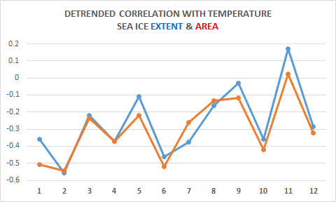
FIGURE 4: TRENDS IN ANTARCTIC SEA ICE EXTENT AND AREA

FIGURE 5: CORRELATION OF ANTARCTIC SEA ICE DECLINE W/GLOBAL WARMING

FIGURE 6: DETRENDED CORRELATION ANALYSIS: ANTARCTIC SEA ICE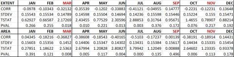

FIGURE 7: SEPTEMBER 2019 UPDATE#1: NORTH: THE ARCTIC

1. This update was added to the post when 2019 data for the important month of September became available. It is noted that due to the extreme seasonal cycle of sea ice extent, the proposed AGW driven decline of sea ice is measured in terms of its seasonal maximum (March in the North and September in the South) and its seasonal minimum (September in the North and February in the South). These seasonal extremes are highlighted in the Figure 7 above and Figure 8 below. Both the EXTENT and AREA measures of sea ice are presented and analyzed.
2. The data for the Arctic (NORTH) appear in Figure 7 above. The temperature data in this chart are UAH lower troposphere temperatures for the North Polar Ocean. They show statistically significant warming trends along with statistically significant decline in sea ice extent for all calendar months suggesting that the decline in sea ice may be driven by AGW and this apparent inverse relationship is generally interpreted in terms of the assumption that global warming by way of fossil fuel emissions is causing a decline in sea ice extent.
3. In the “EXTENT CORR” column of Figure 7 we find the statistically significant negative correlations between temperature and sea ice extent needed to support the causal relationship that AGW drives the decline in sea ice extent. However, since correlation derives from both shared trends and responsiveness, it is necessary to remove the shared trend effect and isolate the effect of responsiveness and these correlations are shown in the detrended correlation column labeled DETCOR.
4. Here, with a sample size of 40, correlations with absolute value greater than ρ=0.464 can be considered statistically significant at α=0.001 as suggested by Valen Johnson in “Revised standards for statistical significance” [LINK] in which he addresses the state of an unacceptable rate of irreproducible results in published research. At the more commonly used error rate of α=0.01, the lowest correlation for statistical significance in this case is ρ=0.358. Using these criteria we find as follows for the Arctic sea ice extent in Figure 7 above:
5. A decline in March Maximum EXTENT is found along with a statistically significant warming trend but the data do not indicate a corresponding decline in March maximum sea ice AREA. Detrended correlation analysis does not show that the decline in March Maximum sea ice extent can be explained in terms of global warming.
6. Declines in both September Minimum sea ice EXTENT and sea ice AREA are found. However, detrended correlation analysis does not show that the observed sea ice decline in EXTENT or in AREA can be explained in terms of temperature trends as no responsiveness relationship is found.
7. The data for the SOUTH (Antarctic) appear in Figure 8 below. No evidence is found of sea ice decline either in the September Maximum or in the February Minimum. The temperature data in this chart are UAH lower troposphere temperatures for the South Polar Ocean. In both of these calendar months we find both extent and area measures of sea ice show a rising trend. An oddity of the detrended correlation of these rising trends of sea ice with ambient temperature shows the odd result that the September maximum area is growing over a period of cooling while February minimum sea ice extent is growing while warming. Such anomalous results point to the importance of geothermal heat in the understanding of sea ice dynamics as explained in related posts [LINK] [LINK] .

FIGURE 8: SEPTEMBER 2019 UPDATE#2: SOUTH: THE ANTARCTIC

THE EISENMAN 2007 PAPER ON INTERMODEL DIFFERENCES ON SEA ICE EXTENT

Eisenman, Ian, Norbert Untersteiner, and J. S. Wettlaufer. “On the reliability of simulated Arctic sea ice in global climate models.” Geophysical Research Letters 34.10 (2007).  While most of the global climate models (GCMs) currently being evaluated for the IPCC Fourth Assessment Report simulate present‐day Arctic sea ice in reasonably good agreement with observations, the intermodel differences in simulated Arctic cloud cover are large and produce significant differences in downwelling longwave radiation. Using the standard thermodynamic models of sea ice, we find that the GCM‐generated spread in longwave radiation produces equilibrium ice thicknesses that range from 1 to more than 10 meters. However, equilibrium ice thickness is an extremely sensitive function of the ice albedo, allowing errors in simulated cloud cover to be compensated by tuning of the ice albedo. This analysis suggests that the results of current GCMs cannot be relied upon at face value for credible predictions of future Arctic sea ice.

BELOW IS THE ORIGINAL POST FOR THE TIME SPAN 1979-2018 THAT INCLUDES ALL TWELVE CALENDAR MONTHS. 

1. In September 2019, the WMO released a report with an alarming list of climate change impacts [LINK] . Included in the many alarming claims made in the report is an extensive and startling evaluation of the decline in sea ice extent in the Arctic and the Antarctic attributed to anthropogenic global warming (AGW).
2. In the report, the WMO lists six concerns about the AGW impact on polar sea ice extent claiming that : (1) From 1979 to 2019, Arctic summer minimum sea ice extent (September) had declined at a rate of 12% per decade; (2) In each of the years 2015, 2016, 2017, 2018, and 2019, the Arctic summer minimum (September) and winter maximum (March) sea ice extents were lower than the 1981-2010 average; (3) The four lowest values for Arctic winter maximum sea ice extent (March) since 1979 are found in the five most recent years 2015 to 2019; (4) Summer sea ice extent in Antarctica (February) reached its lowest and second lowest extents in 2017 and 2018 respectively; (5) The second lowest winter maximum sea ice extent in Antarctica (September) since 1979 was recorded in 2017. (6) Most remarkably, Antarctic summer minimum (February) and winter maximum (September) sea ice extent in the period 2015-2019 are well below the 1981-2010 average. This surprising result is in sharp contrast with the rising trends for both winter and summer seen in the periods 1979-2018 and 2011-2015. Briefly, a catastrophic sea ice decline is claimed for both poles and the decline is attributed to AGW with the implication that these declines can and must be attenuated by following the UN mandated climate action procedures.
3. In this post we show that the available sea ice data from January 1979 to December 2018 are inconsistent with the claims made in the WMO September 2019 report [LINK] .
4.  Figure 1 shows that Arctic sea ice extent has been in decline in all twelve calendar months and that these decline rates are statistically significant. A somewhat weaker decline is seen in the sea ice area. The difference between extent and area has to do with how the satellite measurement grids are tallied [LINK] . To avoid controversy on the choice of sea ice measure, both extent and area are presented in this analysis.
5. The simple fact that sea ice has been in decline during a time when AGW was in process does not in itself imply that AGW is the cause of the decline. Evidence for such causation must be shown to exist in the data. In Figure 2 we present the correlation between UAH lower troposphere temperature over North Polar Ocean against sea ice extent (and area). If rising air temperature is causing a decline in sea ice we would expect to see a negative correlation between temperature and sea ice extent (and area). And that is what we see in Figure 2 where strong and statistically significant negative correlations are found between temperature and sea ice extent (and area).
6. However, it is known that correlations between time series data arise from both shared trends over the full span as well as from responsiveness of the object variable to changes in the explanatory variable at a given finite time scale. Only the second source of correlation has a causation interpretation. In Figure 3, the correlation derived from responsiveness at an annual time scale is tested by removing the correlation due to shared trends. The detrended correlation analysis presented in Figure 3 paints a very different picture. Although statistically significant detrended correlation is found in six of the twelve calendar months, no correlation is found at an annual time scale between temperature and sea ice extent in the two critical months of seasonal minimum sea ice extent in September (where the strongest decline is seen) and seasonal maximum sea ice extent in March. Therefore, we find no evidence for the high profile claim by the WMO [LINK] and climate science in general that AGW is driving down September minimum and March maximum sea ice extent in the Arctic. It is proposed that all sources of heat must be considered, in particular the extensive geothermal heat sources of the Arctic region described in a related post [LINK] must be considered instead of arbitrary attribution to AGW derived from the bias in climate science in which all surface phenomena are seen in the context of AGW.
7. The corresponding analysis for Antarctic sea ice in conjunction with lower troposphere temperatures for the South Polar oceans is presented in Figure 4, Figure 5, and Figure 6. Here the attribution of observed changes to AGW is much weaker particularly so in light of the trend  values which show overall gain and not loss in sea ice extent and area; and none of the correlations between changes in sea ice extent (and area) and lower troposphere temperature are statistically significant.
8. In light of the above, the claim by the WMO of horrific and alarming impacts of AGW on Arctic and Antarctic sea ice extent are not found to have any basis in the data. An additional consideration is the language and peculiarity of the evidence of AGW impact that appear to indicate a circular reasoning effort to find some kind of peculiarity in the data so that an AGW impact can be claimed. A summary of the WMO statement about sea ice is reproduced below.
9. WMO: Six concerns about AGW impact on polar sea ice extent: (1) From 1979 to 2019, Arctic summer minimum sea ice extent (September) had declined at a rate of 12% per decade; (2) In each of the years 2015, 2016, 2017, 2018, and 2019, the Arctic summer minimum (September) and winter maximum (March) sea ice extents were lower than the 1981-2010 average; (3) The four lowest values for Arctic winter maximum sea ice extent (March) since 1979 are found in the five most recent years 2015 to 2019; (4) Summer sea ice extent in Antarctica (February) reached its lowest and second lowest extents in 2017 and 2018 respectively; (5) The second lowest winter maximum sea ice extent in Antarctica (September) since 1979 was recorded in 2017. (6) Most remarkably, Antarctic summer minimum (February) and winter maximum (September) sea ice extent in the period 2015-2019 are well below the 1981-2010 average. This surprising result is in sharp contrast with the rising trends for both winter and summer seen in the periods 1979-2018 and 2011-2015.

[RELATED POST: WMO 2019]

[RELATED POST: ARCTIC SEA ICE]

[RELATED POST ANTARCTIC SEA ICE]

[LINK TO HOME PAGE]

UNITED IN SCIENCE

HIGH-LEVEL SYNTHESIS REPORT OF LATEST CLIMATE SCIENCE INFORMATION

Climate change is the defining challenge of our time.

By the Science Advisory Group of the UN Climate Action Summit 2019 (SAGUCAS2019). The SAGUCAS2019 have convened the report United in Science to assemble the key scientific findings of recent work undertaken by major partner organizations in the domain of global climate change research, including the:

1. World Meteorological Organization (WMO)
2. UN Environment
3. Global Carbon Project
4. The Intergovernmental Panel on Climate Change
5. Future Earth
6. Earth League
7. Global Framework for Climate Services.

1. United in Science is a synthesis of the key findings from several more detailed reports provided by these partners in a transparent envelope. This important document by the United Nations and global partner organizations, prepared under the auspices of the Science Advisory Group of the Climate Action Summit, features the latest critical data and scientific findings on the climate crisis. It shows how our climate is already changing and highlights the far-reaching and dangerous impacts that will unfold for generations to come. Science informs governments in their decision-making and commitments. I urge leaders to heed these facts, unite behind the science and take ambitious, urgent action to halt global heating and set a path towards a safer, more sustainable future for all.
2. The UN Climate Action Summit 2019 Science Advisory Group called for this High Level Synthesis Report, to assemble the key scientific findings of recent work undertaken by major partner organizations in the domain of global climate change research, including the World Meteorological Organization, UN Environment, Global Carbon Project, the Intergovernmental Panel on Climate Change, Future Earth, Earth League and the Global Framework for Climate Services. The Report provides a unified assessment of the state of our Earth system under the increasing influence of anthropogenic climate change, of humanity’s response thus far and of the far-reaching changes that science projects for our global climate in the future. The scientific data and findings presented in the report represent the very latest authoritative information on these topics. It is provided as a scientific contribution to the UN Climate Action Summit 2019, and highlights the urgent need for the development of concrete actions that halt the worst effects of climate change.
3. The Synthesis Report is an example of the international scientific community’s commitment to strategic collaboration in order to advance the use of scientific evidence in global policy, discourse and action. The Science Advisory Group will remain committed to providing its expertise to support the global community in tackling climate change on the road to COP 25 in Santiago and beyond.
4. This report has been compiled by the World Meteorological Organization under the auspices of the SAGUCAS2019, to bring together the latest climate science related updates from a group of key global partner organizations – The World Meteorological Organization (WMO), UN Environment (UNEP), Intergovernmental Panel on Climate Change (IPCC), Global Carbon Project, Future Earth, Earth League and the Global Framework for Climate Services (GFCS). The content of each chapter of this report is attributable to published information from the respective organizations. Overall content compilation of this material has been carried out by the World Meteorological Organization.
5. Warmest five-year period on record: The average global temperature for 2015–2019 is on track to be the warmest of any equivalent period on record. It is currently estimated to be 1.1°Celsius (± 0.1 °C) above pre-industrial (1850–1900) times and 0.20 ±0.08 °C warmer than the global average temperature for 2011–2015. The 2015-2019 five-year average temperatures were the highest on record for large areas of the United States, including Alaska, eastern parts of South America, most of Europe and the Middle East, northern Eurasia, Australia, and areas of Africa south of the Sahara. July 2019 was the hottest month
   

   

    

6. Sea-level rise is accelerating, sea water is becoming more acidic
   The observed rate of global mean sea-level rise increased from 3.04 millimeters per year (mm/yr) during the period 1997–2006 to approximately 4 mm/yr during the period 2007–2016. The accelerated rate in sea level rise as shown by altimeter satellites is attributed to the increased rate of ocean warming and land ice melt from the Greenland and West Antarctica ice sheets. The ocean absorbs nearly 25% of the annual emissions of anthropogenic CO2 thereby helping to alleviate the impacts of climate change on the planet. The absorbed CO2 reacts with seawater and increases the acidity of the ocean. Time series of altimetry-based global mean sea level from January 1993–May 2019. The thin black line is a quadratic function showing the mean sea-level rise acceleration. Data source: European Space Agency (ESA) Climate Change Initiative (CCI) sea-level data until December 2015, extended by data from the Copernicus Marine Service (CMEMS) as of January 2016 and near realtime Jason-3 as of April 2019. Observations show an overall increase of 26% in ocean acidity since the beginning of the industrial era. The ecological cost to the ocean, however, is high, as the changes in acidity are linked to shifts in other carbonate chemistry parameters, such as the saturation state of aragonite. This process, detrimental to marine life and ocean services, needs to be constantly monitored through sustained ocean observations.
   
7. Continued decrease of sea ice 
   The long-term trend over the 1979-2018 period indicates that Arctic summer sea-ice extent has declined at a rate of approximately 12% per decade. In every year from 2015 to 2019, the Arctic average summer minimum and winter maximum sea-ice extent were well below the 1981–2010 average. The four lowest values for winter sea-ice extent occurred in these five years. Summer sea ice in Antarctica reached its lowest and second lowest extent on record in 2017 and 2018, respectively. The second lowest winter extent ever recorded was also experienced in 2017. Most remarkably sea ice extent values for the February minimum (summer) and September maximum (winter) in the period from 2015-2019 have been well below the 1981-2010 average since 2016. This is a sharp contrast with the 2011-2015 period and the long term 1979-2018 values that exhibited increasing trends in both seasons.
8. Continued decrease land ice mass: Overall, the amount of ice lost annually from the Antarctic ice sheet increased at least six-fold between 1979 and 2017. The total mass loss from the ice sheet increased from 40 Gigatons (Gt) average per year in 1979–1990 to 252 Gt per year in 2009–2017. Sea level rise contribution from Antarctica averaged 3.6 ± 0.5 mm per decade with a cumulative 14.0 ± 2.0 mm since1979. Most of the ice loss takes place by melting the ice shelves from below, due to incursions of relatively warm ocean water, especially in West Antarctica and to a lesser extent along the Peninsula and in East Antarctica.
9. Analysis of long-term variations in glacier mass often relies on a set of global reference glaciers, defined as sites with continuous high-quality in situ observations of more than 30 years. Results from these time series are, however, only partly representative for glacier mass changes at the global scale as they are biased to well-accessible regions such as the European Alps, Scandinavia and the Rocky Mountains. Nevertheless, they provide direct information on the year-to-year variability in glacier mass balance in these regions. For the period 2015–2018, data from the World Glacier Monitoring Service (WGMS) reference glaciers indicate an average specific mass change of − 908 mm water equivalent per year. This depicts a greater mass loss than in all other five-year periods since 1950, including the 2011-2015 period. Warm air from a heatwave in Europe in July 2019 reached Greenland, sending temperature and surface melting to record levels.
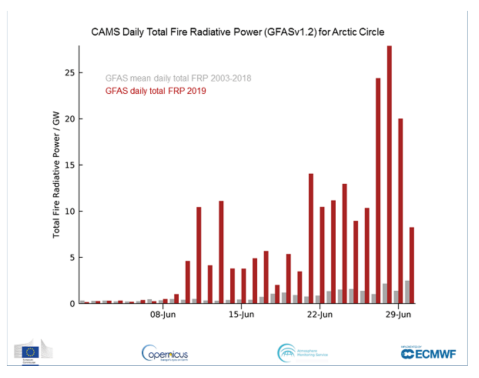
10. Intense heatwaves and wild fires: The Fire Radiative Power (Gigawats)– a measure of heat output from wildfires shown in June for 2019 (red) and the 2003–2018 average (grey) (Source: Copernicus Atmospheric Monitoring Services (CAMS)). Number of undernourished people in the world, 2015–2018 (FAO, IFAD, UNICEF and WHO, 2019. Heatwaves were the deadliest meteorological hazard in the 2015–2019 period, affecting all continents and setting many new national temperature records. Summer 2019 saw unprecedented wildfires in the Arctic region. In June alone, these fires emitted 50 megatons (Mt) of carbon dioxide into the atmosphere. This is more than was released by Arctic fires in the same month from 2010 to 2018 put together. There were multiple fires in the Amazon rainforest in 2019, in particular in August.  The Fire Radiative Power (Gigawats)– a measure of heat output from wildfires shown in June for 2019 (red) and the 2003–2018 average (grey) (Source: Copernicus Atmospheric Monitoring Services (CAMS)). Number of undernourished people in the world, 2015–2018 (FAO, IFAD, UNICEF and WHO, 2019 
11. Costly tropical cyclones. Overall, the largest economic losses were associated with tropical cyclones. The 2018 season was especially active, with the largest number of tropical cyclones of any year in the twenty-first century. All Northern Hemisphere basins experienced above average activity – the Northeast Pacific recorded its largest Accumulated Cyclone Energy (ACE) value ever. The 2017 Atlantic hurricane season was one of the most devastating on record with more than US$ 125 billion in losses associated with Hurricane Harvey alone. Unprecedented back-to-back Indian Ocean tropical cyclones hit Mozambique in March and April 2019.
12. Food insecurity increasing. According to the Food and Agriculture Organization of the United Nations (FAO) report on the State of Food Security and Nutrition in the World, climate variability and extremes are among the key drivers behind the recent rises in global hunger after a prolonged decline and one of the leading contributors to severe food crises. Climate variability and extremes are negatively affecting all dimensions of food security – food availability, access, utilization and stability. The frequency of drought conditions from 2015–2017 show the impact of the 2015–2016 El Niño on agricultural vegetation. The following map shows that large areas in Africa, parts of central America, Brazil and the Caribbean, as well as Australia and parts of the Near East, experienced a large increase in frequency of drought conditions in 2015–2017 compared to the 14-year average. 

Percentage of time (dekad is a 10-day period) with active vegetation when the Anomaly Hot Spots of Agricultural Production (ASAP) was signaling possible agricultural production anomalies according to NDVI (Normalized Difference Vegetation Index) for more than 25% of the crop areas in 2015–2017 (FAO, IFAD, UNICEF, WFP and WHO, 2018) 

13. Overall risk of climate-related illness or death increasing: Based on data and analysis from the World Health Organisation (WHO), between 2000 and 2016, the number of people exposed to heatwaves was estimated to have increased by around 125 million. The average length of individual heatwave events was 0.37 days longer, compared to the period between 1986 and 2008, contributing to an increased risk of heat-related illness or death. 

14. Gross domestic product is falling in developing countries due to increasing temperatures. The International Monetary Fund found that for a medium and low-income developing country with an annual average temperature of 25 °C, the effect of a 1 °C increase in temperature is a fall in growth by 1.2%. Countries whose economies are projected to be hard hit by an increase in temperature accounted for only about 20% of global Gross Domestic Product (GDP) in 2016. But they are home to nearly 60% of the global population, and this is expected to rise to more than 75% by the end of the century.

15. Global Fossil CO2 Emissions. CO​Emissions from fossil fuel use continue to grow by over 1% annually and 2% in 2018 reaching a new high. Growth of coal emissions resumed in 2017.

16. Greenhouse Gas Concentrations: Increases in CO₂ concentrations continue to accelerate. Current levels of CO₂, CH₄ and N₂O represent 146%, 257% and 122% respectively of pre-industrial levels (pre-1750)​. 

17. Emissions Gap: Global emissions are not estimated to peak by 2030, let alone by 2020. Implementing current unconditional NDCs (INDCs) would lead to a global mean temperature rise between   2.9 °C and 3.4 °C by 2100 relative to pre-industrial levels, and continuing thereafter. The current level of NDC (INDC) ambition needs to be roughly tripled for emission reduction to be in line with the 2 °C goal and increased five-fold for the 1.5 °C goal. Technically it is still possible to bridge the gap​.

18. IPCC: Intergovernmental Panel on Climate Change 2018 & 2019 Special Reports: Limiting temperature to 1.5 °C above pre-industrial levels would go hand-in-hand with reaching other world goals such as achieving sustainable development and eradicating poverty. Climate change puts additional pressure on land and its ability to support and supply food, water, health and wellbeing. At the same time, agriculture, food production, and deforestation are major drivers of climate change​

19. Climate Insights: Growing climate impacts increase the risk of crossing critical tipping points. There is a growing recognition that climate impacts are hitting harder and sooner than climate assessments indicated even a decade ago. Meeting the Paris Agreement requires immediate and all-inclusive action encompassing deep de-carbonization complemented by ambitious policy measures, protection and enhancement of carbon sinks and biodiversity, and effort to remove CO2 from the atmosphere​

COMMENTS ON THE WMO UNITED IN SCIENCE REPORT, SEPTEMBER, 2019

COMMENT#1: ITEM#5: WARMEST 5-YEAR PERIOD ON RECORD:  The AGW issue is understood only as the effect of rising atmospheric CO2 on a long term warming trend. In that context, the finding that the years 2015, 2016, 2017, 2018 have set a temperature record in terms of annual mean temperature has no interpretation. Also, the inclusion of the year 2019 in this record temperature claim with temperatures for 4 calendar months of 2019 still in the future is not possible. An additional consideration is that the 2015-2016 El Nino event was one of the strongest on record and the 2017 & 2018 La Ninas were exceptionally weak as seen in the chart below provided by Meteorologist Jan Null. It is precisely because of such anomalous temperature events that are unrelated to long term trends that temperature events do not serve as evidence of long term trends and AGW, that is, CO2 driven warming, relates only to long term temperature trends and not to temperature events. Particularly egregious is the inclusion of these ENSO event years in a an assessment of CO2 driven long term warming of AGW climate change. The “warmest 5-year” argument for AGW is therefore irrelevant and possibly motivated by bias and activism and not by objective and unbiased scientific inquiry.

COMMENT #2: ITEM#6: SEA LEVEL RISE IS ACCELERATING 

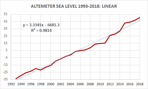
Below are three charts depicting altimeter sea level rise data 1993-2018. The first chart plots sea level against time in years along with a first order linear regression line shown in dots. A statistically significant linear trend is seen with an overall average rate of sea level rise estimated at 3.334 mm/year equivalent to a one meter rise in sea level every 300 years. However, some divergences from a purely linear trend are apparent in the regression line both higher and lower. These divergences are made more clear in the second chart that plots the residuals – the difference between the data and the regression line. In terms of the acceleration issue, we would expect to find that the residuals would be mostly negative at the beginning of the series and gradually rise to above the regression line toward the end of the series. But this is not the case. Instead what we find is that there are large positive differences at the beginning and at the end but with negative differences in the middle from 1998-2014. These data do not support sustained acceleration in sea level rise across the time span studied. That conclusion is supported by the third chart that plots 5-year trends in sea level. Here we find that all the trends are positive implying that over this period sea level rises but does not fall. However, the rate of sea level rise declines from 2001 to 2011 and rises thereafter until 2015 but then declines again toward the end from 2015 to 2018. These data do not provide convincing evidence that sea level rise is accelerating. It is also noted that acceleration in sea level rise, though often presented by the WMO and the IPCC as evidence of human cause, does not in itself prove human cause because the additional data relationships needed in that argument are assumed but not provided, possibly because they don’t exist. For example, if acceleration in sea level rise proves human cause by way of fossil fuel emissions, how does one explain rapid acceleration in sea level rise in the Eemian [LINK] ? To prove human cause of sea level rise by way of fossil fuel emissions; and to support the assumption that climate action in the form of reducing fossil fuel emissions will attenuate sea level rise, a relationship between emissions and sea level rise must exist in the data. Such a relationship was presented in Clark, Peter U., et al. “Sea-level commitment as a gauge for climate policy.” Nature Climate Change 8.8 (2018): 653; However, it is shown in a related post [LINK] that the correlation between cumulative emissions and cumulative sea level rise presented by Clark et al contains neither time scale nor degrees of freedom. This correlation is spurious and has no interpretation in terms of human cause of the observed gradual late Holocene sea level rise. In a related post we show that when these statistics errors in Clark 2018 are corrected, the correlation relating sea level rise to emissions disappears. No evidence is found in the data that the slow residual sea level rise of the late Holocene can be attributed to fossil fuel emissions or that climate action in the form of reducing fossil fuel emissions will attenuate the rate of sea level rise [LINK] . It should also be noted that a sustained and pressing issue in climate science has been the firmly held belief, particularly since the dramatic collapse of the Larsen B ice shelf in 2002 that was arbitrarily attributed to AGW, that some kind of Antarctica ice melt event by way of fossil fuel emissions will cause catastrophic sea level rise [LINK] . The catastrophic sea level rise obsession of climate science with Antarctica is puzzling in the context of known sources of geothermal heat and geological activity that control ice melt dynamics of that continent [LINK] . 

COMMENT #3: ITEM#6: SEA LEVEL RISE IS ACCELERATING AND SEA WATER IS BECOMING MORE ACIDIC. 

There have been significant and catastrophic ocean acidification events by CO2 in the past as recorded in paleo climatology.  However, in these events the source of the carbon dioxide was not the atmosphere but geological and from the ocean itself. No paleoclimate record exists to establish the ability of the atmosphere to acidify the ocean. In terms of relative mass, the ocean is 99.62% and the atmosphere 0.38% of their combined mass. Ocean acidification events of the past are understood in terms of ocean floor and geological sources of carbon and not in terms of atmospheric effects [LINK] . The theory of atmosphere driven ocean acidification is studied with correlation analysis in a related post. No evidence is found to attribute changes in oceanic inorganic carbon to fossil fuel emissions [LINK] . It is likely that the ocean acidification hypothesis entered the climate change narrative by way of the PETM climate change event when extensive and devastating ocean acidification had occurred as described in a related post [LINK] . However, there is no parallel between PETM and AGW that can be used to relate the characteristics of one to those of the other. In the case of ocean acidification in the PETM event, the source of carbon was a monstrous release of geological carbon from the ocean floor or from the mantle. The event caused the ocean to lose all its elemental oxygen by way of carbon oxidation and undergo significant decline in pH. Much of the carbon dioxide was also vented to the atmosphere and that caused atmospheric CO2 to rise precipitously.  But this correspondence of ocean acidification in the presence of rising atmospheric CO2 does not apply to AGW. Whereas PETM started in the ocean and spread to the atmosphere, the AGW event started in the atmosphere and is thought to have spread to the oceans. The evidence presented in a related post  [LINK]  does not support this hypothesis. The effort by climate change scientists to relate all observed changes on the surface of the planet to fossil fuel emissions likely derives from an activism bias to promote fossil fueled catastrophe that corrupts the process of unbiased scientific inquiry in this field [LINK] . 

COMMENT #4: CONTINUED DECREASE OF SEA ICE

1. WMO: Six concerns about AGW impact on polar sea ice extent: (1) From 1979 to 2019, Arctic summer minimum sea ice extent (September) had declined at a rate of 12% per decade; (2) In each of the years 2015, 2016, 2017, 2018, and 2019, the Arctic summer minimum (September) and winter maximum (March) sea ice extents were lower than the 1981-2010 average; (3) The four lowest values for Arctic winter maximum sea ice extent (March) since 1979 are found in the five most recent years 2015 to 2019; (4) Summer sea ice extent in Antarctica (February) reached its lowest and second lowest extents in 2017 and 2018 respectively; (5) The second lowest winter maximum sea ice extent in Antarctica (September) since 1979 was recorded in 2017. (6) Most remarkably, Antarctic summer minimum (February) and winter maximum (September) sea ice extent in the period 2015-2019 are well below the 1981-2010 average. This surprising result is in sharp contrast with the rising trends for both winter and summer seen in the periods 1979-2018 and 2011-2015.
2. RESPONSE: The data show that Antarctic sea ice extent is not declining and if anything it is expanding. Sea ice decline is found in the Arctic particularly so in the summer minimum month of September. However, the correlation needed to attribute the decline to global warming is not found in the data either for the summer minimum in September or for the winter maximum in March. Details provided in a related post [LINK] .

[HOME PAGE]

[THE REMAINING CARBON BUDGET]

[THE REMAINING CARBON BUDGET ANOMALY EXPLAINED]

DR. GLEN PETERS: “THE CARBON BUDGET CONCEPT IS SEDUCTIVELY SIMPLE BUT HAS LARGE UNCERTAINTIES AND MYSTERIOUS COMPLEXITIES”.

HERE WE SHOW THAT THESE UNCERTAINTIES AND COMPLEXITIES ARE THE PRODUCTS OF A FATAL STATISTICAL FLAW IN CARBON BUDGET MATHEMATICS. 

PART 1: HOW THE TCRE CARBON BUDGET IS USED IN CLIMATE SCIENCE

Carbon budget accounting is based on the TCRE  (Transient Climate Response to Cumulative Emissions). It is derived from the observed correlation between temperature and cumulative emissions. A comprehensive explanation of an application of this relationship in climate science is found in the  IPCC SR 15 2018. This IPCC description is quoted below in paragraphs #1 to #7 where the IPCC describes how climate science uses the TCRE for climate action mitigation of AGW in terms of the so called the carbon budget. Also included are some of difficult issues in carbon budget accounting and the methods used in their resolution.

1. Mitigation requirements can be quantified using the carbon budget approach that relates cumulative CO₂ emissions to global mean temperature in terms of the TCRE. Robust physical understanding underpins this relationship.
2. But uncertainties become increasingly relevant as a specific temperature limit is approached. These uncertainties relate to the transient climate response to cumulative carbon emissions (TCRE), non-CO₂ emissions, radiative forcing and response, potential additional Earth system feedbacks (such as permafrost thawing), and historical emissions and temperature. 
3. Cumulative CO₂ emissions are kept within a budget by reducing global annual CO₂ emissions to net zero. This assessment suggests a remaining budget of about 420 GtCO₂ for a two-thirds chance of limiting warming to 1.5°C, and of about 580 GtCO₂ for an even chance (medium confidence). 
4. The remaining carbon budget is defined here as cumulative CO₂ emissions from the start of 2018 until the time of net zero global emissions for global warming defined as a change in global near-surface air temperatures. Remaining budgets applicable to 2100 would be approximately 100 GtCO₂ lower than this to account for permafrost thawing and potential methane release from wetlands in the future, and more thereafter. These estimates come with an additional geophysical uncertainty of at least ±400 GtCO₂, related to non-CO₂ response and TCRE distribution. Uncertainties in the level of historic warming contribute ±250 GtCO₂. In addition, these estimates can vary by ±250 GtCO₂ depending on non-CO₂ mitigation strategies as found in available pathways. {2.2.2, 2.6.1}
5. Staying within a remaining carbon budget of 580 GtCO₂ implies that CO₂ emissions reach carbon neutrality in about 30 years, reduced to 20 years for a 420 GtCO₂ remaining carbon budget. The ±400 GtCO₂ geophysical uncertainty range surrounding a carbon budget translates into a variation of this timing of carbon neutrality of roughly ±15–20 years. If emissions do not start declining in the next decade, the point of carbon neutrality would need to be reached at least two decades earlier to remain within the same carbon budget. {2.2.2, 2.3.5} 
6. Non-CO₂ emissions contribute to peak warming and thus affect the remaining carbon budget. The evolution of methane and sulfur dioxide emissions strongly influences the chances of limiting warming to 1.5°C. In the near-term, a weakening of aerosol cooling would add to future warming, but can be tempered by reductions in methane emissions (high confidence). Uncertainty in radiative forcing estimates (particularly aerosol) affects carbon budgets and the certainty of pathway categorizations. Some non-CO₂ forcers are emitted alongside CO₂, particularly in the energy and transport sectors, and can be largely addressed through CO₂ mitigation. Others require specific measures, for example, to target agricultural nitrous oxide (N₂O) and methane (CH₄), some sources of black carbon, or hydrofluorocarbons. In many cases, non-CO₂ emissions reductions are similar in 2°C pathways, indicating reductions near their assumed maximum potential by integrated assessment models. Emissions of N₂O and NH₃ increase in some pathways with strongly increased bioenergy demand. {2.2.2, 2.3.1, 2.4.2, 2.5.3} 

[RELATED POST ON THE REMAINING CARBON BUDGET]

PART 2: THE TCRE PROPORTIONALITY IS A SPURIOUS STATISTIC AND THEREFORE THE CARBON BUDGET IS AN ILLUSORY TOOL OF CLIMATE ACTION

1. The computation of cumulative values requires the use of the same source data item in the computation of more than one cumulative value. This replication implies that there is an information overlap among the cumulative values. The information lost in this manner can be represented in terms of the multiplicity in the use of the time series data when constructing the series of cumulative values. The repeated use of the same source data for computing more than one cumulative value reduces the effective value of the sample size N. Here we present a procedure for estimating the average value of the multiplicity for any sample size and thereby to estimate the effective sample size EFFN in the cumulative series.
2. The last value in the source series is used only once but all of the other values are used more than once. Under these conditions the statistical significance of the correlation between two time series cannot be evaluated regardless of the magnitude of the correlation coefficient.
3. If the summation starts at K=2, the series of cumulative values of a time series X of length N is computed as Σ(X1 to X2), Σ(X1 to X3), Σ(X1 to X4), Σ(X1 to X5) … Σ(X1 to XN-3), Σ(X1 to XN-2), Σ(X1 to XN-1), Σ(X1 to XN).
4. In these N-K+1=N-1 cumulative values, X(N) is used once, X(N-1) is used twice, X(N-2) is used three times, X(N-3) is used four times, X(4) is used N-3 times, X(3) is used N-2 times, X(2) is used N-1 times , and X(1) is also used N-1 times.
5. In general, each of the first K data items will be used N-K+1 times. Thus, the sum of the multiples for the first K data items may be expressed as K*(N-K+1). The multiplicities of the remaining N-K data items form a sequence of integers from one to N-K and their sum is (N-K)*(N-K+1)/2. Therefore, the average multiplicity of the N data items in the computation of cumulative values may be expressed as:
6. AVERAGE-MULTIPLE = [(K*(N-K+1) + (N-K)*(N-K+1)/2]/N. Since multiplicity of use reduces the effective value of the sample size we can express the effective sample size as: EFFN = N/(AVERAGEMULTIPLE) = (N^2)/(K*(N-K+1) + (N-K)*(N-K+1)/2).
7. The usual procedure in the TCRE computation is to use K=2 in which case, EFFN = 1.988. This means that the effective  value of the sample size is less than two  EFFN<2, and that therefore the time series of cumulative values has no degrees of freedom computed as DF=EFFN-2. This is the essence of the statistics issue with the TCRE and the carbon budget procedure that uses the TCRE.
8. The anomalies and oddities with the carbon budget that climate science struggles to rationalize in terms of “radiative forcings of non-CO₂ emissions and Earth system feedbacks such as permafrost thawing are really the creation of a statistics error consisting of the failure to correct the sample size for multiplicity. This failure creates a faux statistical significance of the correlation coefficient and the TCRE regression coefficient that does not actually exist. 
9. To be able to determine the statistical significance of the correlation coefficient it is necessary that the degrees of freedom (DF) computed as EFFN -2 should be a positive integer. This condition is not possible for a sequence of cumulative values that begins with Σ(X1 to X2) where EFFN=1.988 and therefore DF=1.988-2≈0. Thus a time series of the cumulative values of another time series has no degrees of freedom. Also, since all time spans from unity to the full span are used in the computation, the time series of cumulative values has no time scale. The essential statistics issue in the TCRE and its carbon budget implications is that a time series of the cumulative values of another time series has neither time scale nor degrees of freedom.
10. EFFN can be increased to values higher than two only by beginning the cumulative series at a later point K>2 in the time series so that the first summation is Σ(X1 to XK) where K>2. In that case, the total multiplicity is reduced and this reduction increases the value of EFFN somewhat but the sample size is reduced by (K-2) and nothing is gained.
11. These relationships provide the theoretical underpinning for for the spuriousness of correlations between cumulative values. The results show that the time series consisting of the cumulative values of another time series contains neither degrees of freedom not time scale. Therefore both the TCRE correlation and carbon budgets derived from that correlation are spurious and illusory. Numerical results derived from such analysis have no interpretation in terms of the phenomena of nature being studied.

DEMONSTRATION OF THE ANOMALOUS NATURE OF THE TCRE

1. An example TCRE computation appears below in Figure 1. The data are annual emissions and mean annual HadCRUT4 temperature reconstructions 1851 to 2015. In the first chart, a value of TCRE=0.0027C/gigaton of emissions is indicated in the source data at an annual time scale but no correlation is found to support that relationship.
2. The relationship between cumulative values is shown in the next chart of Figure 1 where TCRE=0.0024C/gigaton of emissions is indicated and supported by a near perfect correlation of ρ=0.9017. The absence of correlation in the source data appears to have been overcome by the use of cumulative values.
3. However, the tabulation under the charts shows that the apparent gain in statistical power is illusory. The effective sample size of a time series of the cumulative values of another time series is EFFN=1.988 yielding negative degrees of freedom of DF=1.988-2 = -0.012. Therefore no conclusion can be made from the spurious and illusory correlation between cumulative values because the time series of cumulative values has neither time scale not degrees of freedom.  It is noted that temperature is cumulative annual warming.
4. Figure 2 shows that a the effective sample size can be increased to EFFN=2.05, thereby yielding a positive degrees of freedom if the summation starts at n=30 but the t-statistic is too low to reject the null hypothesis that the hypothesized correlation does not exist.
5. Figure 3  is a split half test of the correlation and TCRE of cumulative values in Figure 1. In the split half test, the first half, the second half. and the mid-half are compared with the full span in terms of correlation and the value of the TCRE coefficient. The comparison shows that there is no agreement between the four TCRE and correlation values for full span, first half, last half, and mid-half. The TCRE is highest for the mid-half (TCRE=0.0035) and lowest for the first half (TCRE=0.0018). The other two values lie somewhere in the middle with full span (TCRE=0.0024) somewhat higher than the second half (TCRE=0.0020). Very little correlation is found in the first half (ρ=0.1784) but the other three spans show statistically significant correlations of ρ=0.9017 for the full span, ρ=0.8860 for the second half and a lower but statistically significant  value of ρ=0.6526 for the mid-half.
6. These differences in the value of the TCRE coefficient at different locations along the time series of cumulative values provide further evidence of its spuriousness and also offers a simple and more realistic explanation for the so called Remaining Carbon Budget (RCB) issue in climate science. The RCB issue is that the carbon budget accounting over the period of the budget is not linear so that for example, if the budget for the next 20 years is 200 gigatons of carbon dioxide, and after 10 years 80 gigatons of cumulative emissions have been produced, the RCB can’t be assumed to be 200-80=120 gigatons because a fresh computation of a carbon budget for the next 10 years typically yields an entirely different non-proportional figure.

7. [HOME PAGE]

   [THE REMAINING CARBON BUDGET]

   [THE REMAINING CARBON BUDGET ANOMALY EXPLAINED]

    

    

8. The correlation and the TCRE value between cumulative warming and cumulative emissions derives from the fact that during a time of long term warming trend, the annual warming values are mostly positive and further that if the rate of warming is rising over the long term the second half of the carbon budget period will contain a greater fraction of positive annual warming values. These values are driven by the fraction of the annual warming values that are positive. In a random series this fraction cannot be assumed to be the same in the two halves of the time series. This is the mundane statistical explanation of the remaining carbon budget issue.
9. In climate science, the Remaining Carbon Budget  issue is interpreted and resolved in esoteric ways and in terms of climate science variables of convenience. These include non CO2 forcings and the so called “earth system factors” such as release of permafrost methane. The analysis presented here suggests a more banal explanation that goes to the heart of the spuriousness of the TCRE correlation. In terms of the statistics presented here, the RCB anomaly is understood simply in terms of the spuriousness of the TCRE coefficient itself and therefore of its non-proportionality across time time span increments.
10. A summary of the correlations observed in the data is shown in Figure 3A. The data do not show a correlation at an annual time scale. The somewhat higher correlation seen at a decadal time scale is found to be spurious and driven by shared trends and not at responsiveness at a decadal time scale. The apparent correlation does not survive into the detrended series. The strong correlation between cumulative values does survive into the detrended series but, as shown above, correlations between cumulative values have no interpretation because of the absence of degrees of freedom and time scale in the data.

FIGURE 1: CORRELATIONS AND TCRE AT K=2

FIGURE 2: CORRELATIONS AND TCRE AT K=30

FIGURE 3: SPLIT HALF TEST OF THE TCRE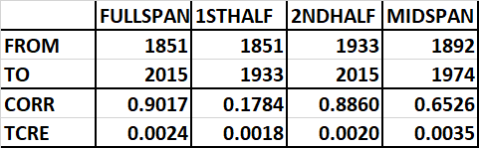

FIGURE 3A: CORRELATION TABLE

1. The anomalous behavior of correlation and the TCRE demonstrated with Figure 1, Figure 2, and Figure 3 above can be understood in terms of how the correlation and TCRE values are generated by the time series. The tabulations in Figure 1 and Figure 2 demonstrate that temperature is cumulative annual warming. It can be shown that the high correlation seen between cumulative emissions and cumulative warming is not an indication of correlation but of a fortuitous sign pattern of annual emissions and annual warming. The sign pattern is that annual emissions are always positive; and, at a time of an overall long term warming trend, annual warming is mostly positive. It is this sign pattern and not real responsiveness of warming to emissions that creates the faux correlation of the TCRE and the faux statistical significance of the TCRE itself. For this reason these values have no interpretation in terms of the phenomena of nature being studied in terms of a responsiveness of warming to emissions.
2. The role of the sign pattern in the TCRE correlation is demonstrated in Figure 4 and Figure 5. The left frame of these figures shows two time series of random numbers X and Y generated by a random number generator such that the X-values in both Figure 4 and Figure 5 are all positive (as in emissions). The Y-values in Figure 4 are completely random with no sign bias. However, the Y-values in Figure 5 are contain a small bias for positive values in the random number generator. The differences between Figure 4 and Figure 5 are therefore understood only in terms of this only difference between them.
3. In both Figure 4 and Figure 5, the left frame shows no sign of correlation between X and Y at an annual time scale verifying that these are random numbers independently generated. However, a significant difference is seen between Figure 4 and Figure 5 in their right frames where the cumulative values of the random numbers are tested graphically for correlation. Here we find a strong positive correlation in Figure 5, where a common positive sign pattern exists with X-values all positive and Y-values with a bias for positive values. No such evidence of a positive correlation exists in Figure 4 where though the X-values are all positive, no positive bias exists in Y-values. Therefore the difference in visual correlation between the two figures is understood on that basis.
4. This demonstration supports the statement above that the TCRE correlation is a creation of a sign pattern. The sign pattern is that emissions are always positive and annual warming is mostly positive during a time of overall warming.
5. that do not show any correlation at all. Their right frames show the relationship between the cumulative values of these completely uncorrelated random numbers.
6. The only difference between Figure 4 and Figure 5 is sign pattern. In Figure 4, the numbers are completely random with no bias for positive values but in Figure 5, a small bias of 5% for positive values is inserted into the random number generator.
7. The strong TCRE linear correlation between cumulative values is seen in Figure 5 but not in Figure 4.  This difference is thus interpreted in terms of the bias for positive values in Figure 5. We conclude from the demonstration in Figure 4 and Figure 5 that the TCRE correlation seen in emissions and warming data is a spurious and illusory creation of a sign pattern. The other, and perhaps more important interpretation of the strong visual correlations seen in Figure 5 is that, under the same conditions and using the same procedures that yield the strong proportionality and statistically significant TCRE value in climate data, the same strong proportionality and statistical significance is seen in random numbers.
8. The only information content of the TCRE is the sign pattern. If the the two time series have a common sign bias, either both positive or both negative, the correlation will be positive. If the the two time series have different sign biases, one positive and the other negative, the correlation will be negative. If the the two time series have no sign bias, no correlation will be found. Therefore, the only information content of the TCRE is the sign pattern and no rational interpretation of such a proportionality exists in terms of a causal relationship that can be used in the construction of carbon budgets. The TCRE carbon budgets of climate science is a a meaningless exercise with an illusory statistic.

FIGURE 4: RANDOM NUMBERS WITHOUT SIGN BIAS 

FIGURE 5: RANDOM NUMBERS WITH SIGN BIAS

[HOME PAGE]

[THE REMAINING CARBON BUDGET]

[THE REMAINING CARBON BUDGET ANOMALY EXPLAINED]

THE UN’S MISSION IS TO IMPOSE CLIMATE ACTION AND THE IPCC’S JOB IS TO PROVIDE A “SCIENTIFIC” RATIONALE FOR CLIMATE ACTION. THE EXPLANATION OF THE ODDITY THAT ALL CLIMATE IMPACTS ARE BAD, THAT ALL BAD THINGS ARE CLIMATE IMPACTS, AND THAT IN THE SCIENCE OF CLIMATE IMPACTS THERE ARE NO GOOD IMPACTS AND NO ATTRIBUTION FAILURES DUE TO UNCERTAINTY IS THAT IPCC SCIENCE IS NOT UNBIASED OBJECTIVE SCIENTIFIC INQUIRY BUT AGENDA DRIVEN TO PROVIDE THE RATIONALE NEEDED  BY THE UN FOR ITS PRE-DETERMINED CLIMATE ACTION AGENDA. IT IS THUS, THAT IN THE AGE OF CLIMATE CHANGE, ALL PROBLEMS – BE IT POLITICAL OR SOCIAL UNREST, WAR, FAMINE, MIGRATION, OR DISEASE – CAN BE FRAMED IN TERMS OF CLIMATE CHANGE AND THEN SOLVED SIMPLY BY CUTTING EMISSIONS. 

A CAUTIONARY TALE ABOUT THE INNER WORKINGS OF THE IPCC AND OF THE EXTREME RISK TO CLIMATE SCIENTISTS OF NOT CONFORMING TO CONSENSUS

ATTRIBUTION OF EXTREME WEATHER TO AGW & THE IPCC

by Roger Pielke Jr published as a Twitter Thread

1. I started studying extreme events in 1993 when I began a post-doc at NCAR on a project focused on lessons learned in Hurricane Andrew & the Midwest floods of 1993. I worked for MickeyGlantz, who was one of my most significant mentors. On March 15, 2006 I received an award from the NAS & gave a lecture to a large audience at the Smithsonian Natural History Museum in DC. My work was viewed to be important, novel and, legitimate. Two months later, An Inconvenient Truth came out, focused on politicizing extreme weather in the climate debate. Extreme weather had always been part of the debate, but it was becoming more central as advocates tried to make climate more relevant to the public.

2. That same May, 2006 I was busy organizing a major international workshop in partnership with MunichRe in Hohenkammer, Germany. We wanted to assess the science of disasters and climate change as input to the upcoming IPCC AR4 report. We wanted to assess scientific understandings on the causes of the trend shown in the data. Why were disasters getting more costly (Chart#1)?  We started by thinking that we’d produce a “consensus/dissensus” report, but wound up with 100% consensus. The workshop [LINK] involved 32 participants & we comissioned 24 background papers. We produced a summary that was published in Science [LINK] [LINK] .
3. The three consensus statements most relevant to this talk are: [Analysis of long term records of disaster losses indicate that societal change and economic development are the principal factors responsible for the increasing losses to date] and [Because of issues related to data quality, the stochastic nature of extreme event impacts, length of time series, and various societal factors present in the disaster loss record, it is still not possible to determine the portion of the increase in damages that can be attributed to climate change due to GHG emissions]. If increasing disaster losses were the result of climate change due to GHG emissions, we could not detect that. It was not a close call, it was unanimous.
4. So when the IPCC AR4 came out, I excitedly looked to see what role this report played in their report. I went to Section “1.3.8.5 Summary of disasters and hazards” only to be blindsided. The report cited “one study” that was apparently at odds with what we had concluded in our assessment. How could 32 experts have all missed this “one study”? The IPCC report said, [1.3.8.5 Summary of Disasters and Hazards: Global losses reveal rapidly rising costs due to extreme weather related events Since the 1970s. One study has found that while the dominant signal remains that of the significant increases in the values of the exposure at risk, once losses are normalized for exposure, there still remains an underlying rising trend].
5. The IPCC AR4 included a mysterious chart [Chart#2] that relates increasing catastrophic losses to rising global temperature. It had never seen that chart before. The reference was [Muir-Wood et al 2006]. It was one of the papers we had commissioned for the Hohenkammer workshop. But I knew it did not include that mysterious graph nor any analysis of temperatures and disasters [Chart#3]. The mysterious temperature to catastrophic loss chart was mysteriously slipped into the IPCC report by one of its authors. who mis-cited it to our Hohenkammer white paper to circumvent an IPCC deadline. He had expected the chart to appear in a future publication but had to mis-cite it to meet the IPCC deadline [Chart#4].
6. That future paper was eventually published well after the IPCC AR4 was released. The paper says [We find insufficient evidence to claim a statistical relationship between global temperature increase and normalized catastrophe losses.] That seemed like a big deal & it was. The Sunday Times did a very good news story on it [Chart#5]. I was interviewed by Christina Larson and it was this interview in which I described the IPCC AR4 irregularities, that resulted in the hit job below [Chart#6] which turned me into a climate “denier”. The Center for American Progress amplified the hit job & continued a campaign of de-legitimization of me & my work. It was relentless. In 2015 Pulitzer Prize winner Paige St. John quoted me innocuously, only to have others calling for her to be fired for doing so. She wrote: [You should come with a warning label. Quoting Roger Pielke will bring a hail storm down on your work from the Guardian, Mother Jones, and Media Matters]. 
7. In 2012 the IPCC Special Report on Managing the Risks of Extreme Events and Disasters to Advance Climate Change Adaptation (SREX) was published. It arrived as the same conclusion as we had at Hohenkammer. Key conclusion: [Long term trends in economic disaster losses adjusted for wealth and population increases have not been attributed to climate change, but a role for climate change has not been excluded. Medium evidence. High agreement] [Chart#7].
8. Despite the IPCC consensus aligned with and drawing upon the work of our  Hohenkammer workshop, the de-legitimization efforts intensified. In 2015 I was the subject of an Congressional “investigation” (w/ 6 other academics), accused of secretly taking Exxon money  [Chart#8]. I cannot describe how penal, professionally and personally, it is to be identified as the subject of a congressional investigation.
   I suppose that was the entire point. I never have taken any money from energy companies. I was cleared in the “investigation [Chart#9]. The reality is Dr. Holdren got caught out while articulating the Al Gore version of disasters & climate change and ignoring the latest IPCC version. I had testified to the IPCC version before the Senate in 2013.

CHART#1 & CHART#2

CHART#3 & CHART#4

CHART#5 & CHART#6

CHART#7 & CHART#8

USCRN TEMPERATURES 2005-2019

1. The chart above is seen in social media and denier blogs with the start year fixed at 2005 and the end year varying from 2017 to 2019 depending on when it was posted. It is meant to show that there is no global warming evident in the data. The chart shows mean temperatures from 114 USCRN station data across the USA. It is claimed that the unique property of this chart is that the start date of 2005 ensures that the UHI (urban heat island) effect has been removed from the data. It is thus argued based on this chart that AGW global warming is a faux creation of UHI because when UHI is removed the evidence for warming disappears from the data. It is further argued that therefore, all datasets that show warming, including the UAH satellite data, are flawed because they show warming when it is now clear that global warming is a creation of UHI. 
2. This post is a critical evaluation of this line of reasoning. First, mean USA temperature cannot be expected to mimic global mean temperature because of the geographical limitation and second, the time span of 15 years is too short for this kind of test as it has been shown in related posts that even strong warming trends do not show consistent monotonic warming year after year but rather that the long term trend is simply the net result of violent warming, cooling, and no trend cycles at decadal and multi-decadal time scales [LINK] [LINK] .
3. FIGURE 1: The chart and regression table in Figure 1 below show UAH global mean temperatures for the eight calendar months January to August over the time span, 2005-2019. The chart appears to show a warming trend and in the corresponding regression table we find p-values<0.05 in four of the eight months with an average p-value for all eight calendar months computed as p-value=0.0488 < 0.05. We conclude that there appears to be some evidence of a warming trend in the UAH global mean temperatures 2005-2019 though it does not appear to be a very strong warming trend.
4. Figure 2: A corresponding analysis of UAH temperatures for the USA lower 48 states is presented in Figure 2. Here the chart appears flat with no indication of a warming trend. The regression table shows very high p-values with an average p-value of 0.2637. The UAH data appear to agree with the USCRN data above that no trend in USA temperatures is evident for the time span 2005-2019.  A comparison of Figure 1 and Figure 2 indicates that the absence of trend in the USCRN temperatures cannot be ascribed to the removal of UHI but with peculiarities of the geographical limitation of the analysis. This comparison does not support the interpretation of the USCRN data in  terms of UHI. In other words, the data do not show that a warming trend was removed because of the exclusion of the UHI effect.
5. Figure 3: That the 15-year time span chosen for the UHI study is too short for drawing conclusions about AGW is shown in the four charts of Figure 3. Here we see large fluctuations in trends for a moving 15-year window as its end year moves through the full span from 1993 to 2019. The overall trend for the full span is therefore understood as a long term warming that accumulates from these violent swings. These charts also provide convincing evidence that 15-year temperature trends do not provide useful information nor information relevant to an empirical test of AGW theory.
6. Figure 4: Shows results for a full span trend analysis of the UAH USA48 data. Very little evidence for statistically significant trends is found in stark contrast with the UAH global temperatures presented in Figure 6 where robust warming trends are found for all eight calendar months January to August with an aveage p-value=0.0002. The comparison of Figure 4 and Figure 6 provide additional evidence that the difference in trends between the USA and the world is not due to UHI but to geographical limitations of the USA-only analysis. It is noted in this context that AGW theory does not claim nor require that all geographical locations should warm at the same rate but only that a long term warming trend should exist in the global mean temperature.
7. SUMMARY AND CONCLUSION: The data presented in the chart at the top of this post are too limited by geography and time span in its trend analysis to have significant implications for AGW where only long term trends in deseasonalized mean global temperature are relevant. Also, the claim that the absence of trend can be attributed to the removal of the UHI effect in 2005 is not supported by the trend profile showing large changes in trends in a moving 15-year window where trends as low or lower are seen prior to 2005. The comparison of USA data from USCRN and UAH does not indicate that the absence of trend since 2005 is due to the removal of the UHI effect because no such intervention exists in the UAH data. 

FIGURE 1: UAH GLOBAL TEMPERATURES 2005-2019 

FIGURE 2: UAH TEMPERATURES FOR USA48 2005-2019

FIGURE 3: TRENDS IN A MOVING 15-YEAR WINDOW: UAH-USA48 1979-2019

FIGURE 4: UAH USA48 FULL SPAN TRENDS: 1979-2019

FIGURE 5: UAH GLOBAL TRENDS IN MOVING 15-YEAR WINDOW 1979-2019

FIGURE 6: UAH GLOBAL FULL SPAN TRENDS 1979-2019

[HOME PAGE]

THIS POST IS A PRESENTATION OF CLIMATE SENSITIVITY RESEARCH PRIOR TO THE CHARNEY-1979 PRESENTATION AND BEFORE THE UNITED NATIONS SEIZED CONTROL OF THIS DISCUSSION THEREAFTER BY CREATING THE UNEP AND THE IPCC.

[LINK TO THE HOME PAGE OF THIS SITE]

1. The history of the Anthropogenic Global Warming Science (AGW) goes back to 1938 when Guy Stewart Callendar published the world’s first AGW paper (using the word artificial instead of anthropogenic). In that paper he noted that the end of the Little Ice Age cooling period [LINK] and the beginning of a warming period coincided with energy innovations that involved the use of coal and other underground hydrocarbon fuels (“fossil fuel”)  and presented an analysis of the warming trend from 1900 to 1938 in terms of atmospheric CO2 measurements from various parts of Europe that showed a rising trend [LINK] . Citing Tyndal and others he computed a regression coefficient of 2.9 for the responsiveness of surface temperature to the natural logarithm of atmospheric CO2 concentration. The corresponding value of the equilibrium climate sensitivity parameter is λ=2°C of warming for each doubling of atmospheric CO2 concentration. It is noteworthy that the Callendar paper did not contain reasons to fear the warming trend nor to take climate action to contain a warming trend that must have been a welcome relief from the Little Ice Age.
2. The Callendar paper was well received and a few more such papers were published in the ensuing years but within a decade of Callendar 1938, the world entered a 30-year cooling period that turned the attention of researchers to global cooling [LINK]
3. The late great Stephen Schneider pointed out that fossil fuel emissions contain not only carbon dioxide but aerosols. Not only do aerosols cause cooling, he said, but while the CO2 warming curve is logarithmic, the aerosol cooling curve is exponential and so it was only a matter of time before the faster and faster aerosol cooling effect would overtake the slower and slower CO2 warming effect.
4. Other similar papers followed with Richard Somerville of Scripps Institute of Oceanography, UC San Diego writing that CO2 induced global warming is self correcting because warming increases cloud formation and clouds reflect sunlight back into space. The AGW issue itself entered a hiatus.
5. The AGW issue was rekindled afresh when the cooling trend ended in the 1970s and by the late 1970s temperatures had begun to rise. A significant event in the resurgence of AGW science was the 1979 presentation by Jule Charney in which he used a climate model to estimate that the value of the climate sensitivity parameter has a mean of λ=3°C with a standard deviation of σ=0.76°C. This uncertainty in the estimate implies a 90% confidence interval of 1.5<λ<4.5. 
6. In later years this estimate of λ was adopted by the IPCC and it became AGW gospel thereafter although in recent years the IPCC has revised the estimate upward to λ=5°C and higher.
7. However, in the intervening years between Callendar and Charney, during the cooling period of the 1950s and 1960s, significant works on climate sensitivity by Syukuro Manabe and others were carried out and their very interesting results published and then apparently forgotten.
8. It is significant that Syukuro Manabe wrote the world’s first climate model and, insult to injury, the now famous Charney estimate of climate sensitivity was estimated using the Manabe climate model.
9. Here we present a summary of climate sensitivity research in these missing years and they are listed in the climate sensitivity bibliography presented below. Some significant works in the missing years include works by Manabe, Wetherald, Plas, Fritz, Ramanathan, and Cess.
10. In Fritz 1963 we find the interesting observation that the CO2 climate sensitivity concept assumes a dry atmosphere because of the common absorption band of 15 μ shared by CO2 and H2O. He estimates the dry climate sensitivity as λ=1.5°C for a doubling of  atmospheric CO2 concentration.
11. In Manabe 1964, he estimates “the role of various gaseous absorbers (i.e., water vapor, carbon dioxide, and ozone), as well as the role of the clouds. He computes thermal equilibrium by removing one element at a time from the portfolio of effects and proposes that the CO2 effect is best understood as λ=2°C for a doubling of  atmospheric CO2 concentration. Interestingly the Manabe 1964 estimate exactly matches the Callendar 1938 estimate.
12. In the now famous paper by Manabe and Wetherald 1967 they state that the climate sensitivity value for CO2 can only be stated  as an initial value problem because of the asymptotic decline with relative humidity. They estimate the dry air climate sensitivity of CO2 as λ=2°C for a doubling of  atmospheric CO2 concentration.
13. Several other interesting works are found in the bibliography below but these results have been superseded by the overarching importance of the Charney estimate that was adopted by the IPCC and also perhaps by the climate policy imperatives of the UN as expressed through its IPCC agency.

BIBLIOGRAPHY

1. 1963: Möller, Fritz. “On the influence of changes in the CO2 concentration in air on the radiation balance of the earth’s surface and on the climate.” Journal of Geophysical Research68.13 (1963): 3877-3886. The numerical value of a temperature change under the influence of a CO₂ change as calculated by Plass is valid only for a dry atmosphere. Overlapping of the absorption bands of CO₂ and H₂O in the range around 15 μ essentially diminishes the temperature changes. New calculations give ΔT = + 1.5° when the CO₂ content increases from 300 to 600 ppm. Cloudiness diminishes the radiation effects but not the temperature changes because under cloudy skies larger temperature changes are needed in order to compensate for an equal change in the downward long‐wave radiation. The increase in the water vapor content of the atmosphere with rising temperature causes a self‐amplification effect which results in almost arbitrary temperature changes, e.g. for constant relative humidity ΔT = +10° in the above mentioned case. It is shown, however, that the changed radiation conditions are not necessarily compensated for by a temperature change. The effect of an increase in CO₂ from 300 to 330 ppm can be compensated for completely by a change in the water vapor content of 3 per cent or by a change in the cloudiness of 1 per cent of its value without the occurrence of temperature changes at all. Thus the theory that climatic variations are effected by variations in the CO₂ content becomes very questionable.
2. 1964: Manabe, Syukuro, and Robert F. Strickler. “Thermal equilibrium of the atmosphere with a convective adjustment.” Journal of the Atmospheric Sciences 21.4 (1964): 361-385. The states of thermal equilibrium (incorporating an adjustment of super-adiabatic stratification) as well as that of pure radiative equilibrium of the atmosphere are computed as the asymptotic steady state approached in an initial value problem. Recent measurements of absorptivities obtained for a wide range of pressure are used, and the scheme of computation is sufficiently general to include the effect of several layers of clouds. The atmosphere in thermal equilibrium has an isothermal lower stratosphere and an inversion in the upper stratosphere which are features observed in middle latitudes. The role of various gaseous absorbers (i.e., water vapor, carbon dioxide, and ozone), as well as the role of the clouds, is investigated by computing thermal equilibrium with and without one or two of these elements. The existence of ozone has very little effect on the equilibrium temperature of the earth’s surface but a very important effect on the temperature throughout the stratosphere; the absorption of solar radiation by ozone in the upper and middle stratosphere, in addition to maintaining the warm temperature in that region, appears also to be necessary for the maintenance of the isothermal layer or slight inversion just above the tropopause. The thermal equilibrium state in the absence of solar insulation is computed by setting the temperature of the earth’s surface at the observed polar value. In this case, the stratospheric temperature decreases monotonically with increasing altitude, whereas the corresponding state of pure radiative equilibrium has an inversion just above the level of the tropopause. A series of thermal equilibriums is computed for the distributions of absorbers typical of different latitudes. According to these results, the latitudinal variation of the distributions of ozone and water vapor may be partly responsible for the latitudinal variation of the thickness of the isothermal part of the stratosphere. Finally, the state of local radiative equilibrium of the stratosphere overlying a troposphere with the observed distribution of temperature is computed for each season and latitude. In the upper stratosphere of the winter hemisphere, a large latitudinal temperature gradient appears at the latitude of the polar-night jet stream, while in the upper statosphere of the summer hemisphere, the equilibrium temperature varies little with latitude. These features are consistent with the observed atmosphere. However, the computations predict an extremely cold polar night temperature in the upper stratosphere and a latitudinal decrease (toward the cold pole) of equilibrium temperature in the middle or lower stratosphere for winter and fall. This disagrees with observation, and suggests that explicit introduction of the dynamics of large scale motion is necessary.
3. 1967: Manabe, Syukuro, and Richard T. Wetherald. “Thermal equilibrium of the atmosphere with a given distribution of relative humidity.” Journal of the Atmospheric Sciences 24.3 (1967): 241-259. [ECS=2]
4. 1969: Budyko, Mikhail I. “The effect of solar radiation variations on the climate of the earth.” tellus 21.5 (1969): 611-619. It follows from the analysis of observation data that the secular variation of the mean temperature of the Earth can be explained by the variation of short-wave radiation, arriving at the surface of the Earth. In connection with this, the influence of long-term changes of radiation, caused by variations of atmospheric transparency on the thermal regime is being studied. Taking into account the influence of changes of planetary albedo of the Earth under the development of glaciations on the thermal regime, it is found that comparatively small variations of atmospheric transparency could be sufficient for the development of quaternary glaciations.
5. 1969: Sellers, William D. “A global climatic model based on the energy balance of the earth-atmosphere system.” Journal of Applied Meteorology 8.3 (1969): 392-400. A relatively simple numerical model of the energy balance of the earth-atmosphere is set up and applied. The dependent variable is the average annual sea level temperature in 10° latitude belts. This is expressed basically as a function of the solar constant, the planetary albedo, the transparency of the atmosphere to infrared radiation, and the turbulent exchange coefficients for the atmosphere and the oceans. The major conclusions of the analysis are that removing the arctic ice cap would increase annual average polar temperatures by no more than 7C, that a decrease of the solar constant by 2–5% might be sufficient to initiate another ice age, and that man’s increasing industrial activities may eventually lead to a global climate much warmer than today.
6. 1971: Rasool, S. Ichtiaque, and Stephen H. Schneider. “Atmospheric carbon dioxide and aerosols: Effects of large increases on global climate.” Science 173.3992 (1971): 138-141. Effects on the global temperature of large increases in carbon dioxide and aerosol densities in the atmosphere of Earth have been computed. It is found that, although the addition of carbon dioxide in the atmosphere does increase the surface temperature, the rate of temperature increase diminishes with increasing carbon dioxide in the atmosphere. For aerosols, however, the net effect of increase in density is to reduce the surface temperature of Earth. Because of the exponential dependence of the backscattering, the rate of temperature decrease is augmented with increasing aerosol content. An increase by only a factor of 4 in global aerosol background concentration may be sufficient to reduce the surface temperature by as much as 3.5 ° K. If sustained over a period of several years, such a temperature decrease over the whole globe is believed to be sufficient to trigger an ice age.
7. 1975: Manabe, Syukuro, and Richard T. Wetherald. “The effects of doubling the CO2 concentration on the climate of a general circulation model.” Journal of the Atmospheric Sciences 32.1 (1975): 3-15. An attempt is made to estimate the temperature changes resulting from doubling the present CO2 concentration by the use of a simplified three-dimensional general circulation model. This model contains the following simplifications: a limited computational domain, an idealized topography, no beat transport by ocean currents, and fixed cloudiness. Despite these limitations, the results from this computation yield some indication of how the increase of CO2 concentration may affect the distribution of temperature in the atmosphere. It is shown that the CO2 increase raises the temperature of the model troposphere, whereas it lowers that of the model stratosphere. The tropospheric warming is somewhat larger than that expected from a radiative-convective equilibrium model. In particular, the increase of surface temperature in higher latitudes is magnified due to the recession of the snow boundary and the thermal stability of the lower troposphere which limits convective beating to the lowest layer. It is also shown that the doubling of carbon dioxide significantly increases the intensity of the hydrologic cycle of the model. 
8. 1976: Cess, Robert D. “Climate change: An appraisal of atmospheric feedback mechanisms employing zonal climatology.” Journal of the Atmospheric Sciences 33.10 (1976): 1831-1843. The sensitivity of the earth’s surface temperature to factors which can induce long-term climate change, such as a variation in solar constant, is estimated by employing two readily observable climate changes. One is the latitudinal change in annual mean climate, for which an interpretation of climatological data suggests that cloud amount is not a significant climate feedback mechanism, irrespective of how cloud amount might depend upon surface temperature, since there are compensating changes in both the solar and infrared optical properties of the atmosphere. It is further indicated that all other atmospheric feedback mechanisms, resulting, for example, from temperature-induced changes in water vapor amount, cloud altitude and lapse rate, collectively double the sensitivity of global surface temperature to a change in solar constant. The same conclusion is reached by considering a second type of climate change, that associated with seasonal variations for a given latitude zone. The seasonal interpretation further suggests that cloud amount feedback is unimportant zonally as well as globally. Application of the seasonal data required a correction for what appears to be an important seasonal feedback mechanism. This is attributed to a variability in cloud albedo due to seasonal changes in solar zenith angle. No attempt was made to individually interpret the collective feedback mechanisms which contribute to the doubling in surface temperature sensitivity. It is suggested, however, that the conventional assumption of fixed relative humidity for describing feedback due to water vapor amount might not be as applicable as is generally believed. Climate models which additionally include ice-albedo feedback are discussed within the framework of the present results.
9. 1978: Ramanathan, V., and J. A. Coakley. “Climate modeling through radiative‐convective models.” Reviews of geophysics16.4 (1978): 465-489. We present a review of the radiative‐convective models that have been used in studies pertaining to the earth’s climate. After familiarizing the reader with the theoretical background, modeling methodology, and techniques for solving the radiative transfer equation the review focuses on the published model studies concerning global climate and global climate change. Radiative‐convective models compute the globally and seasonally averaged surface and atmospheric temperatures. The computed temperatures are in good agreement with the observed temperatures. The models include the important climatic feedback mechanism between surface temperature and H₂O amount in the atmosphere. The principal weakness of the current models is their inability to simulate the feedback mechanism between surface temperature and cloud cover. It is shown that the value of the critical lapse rate adopted in radiative‐convective models for convective adjustment is significantly larger than the observed globally averaged tropospheric lapse rate. The review also summarizes radiative‐convective model results for the sensitivity of surface temperature to perturbations in (1) the concentrations of the major and minor optically active trace constituents, (2) aerosols, and (3) cloud amount. A simple analytical model is presented to demonstrate how the surface temperature in a radiative‐convective model responds to perturbations.
10. 1985: Wigley, Thomas ML, and Michael E. Schlesinger. “Analytical solution for the effect of increasing CO2 on global mean temperature.” Nature 315.6021 (1985): 649. Increasing atmospheric carbon dioxide concentration is expected to cause substantial changes in climate. Recent model studies suggest that the equilibrium warming for a CO2 doubling (Δ T2×) is about 3–4°C. Observational data show that the globe has warmed by about 0.5°C over the past 100 years. Are these two results compatible? To answer this question due account must be taken of oceanic thermal inertia effects, which can significantly slow the response of the climate system to external forcing. The main controlling parameters are the effective diffusivity of the ocean below the upper mixed layer (κ) and the climate sensitivity (defined by Δ T2×). Previous analyses of this problem have considered only limited ranges of these parameters. Here we present a more general analysis of two cases, forcing by a step function change in CO2 concentration and by a steady CO2 increase. The former case may be characterized by a response time which we show is strongly dependent on both κ and Δ T2×. In the latter case the damped response means that, at any given time, the climate system may be quite far removed from its equilibrium with the prevailing CO2 level. In earlier work this equilibrium has been expressed as a lag time, but we show this to be misleading because of the sensitivity of the lag to the history of past CO2 variations. Since both the lag and the degree of disequilibrium are strongly dependent on κ and Δ T2×, and because of uncertainties in the pre-industrial CO2 level, the observed global warming over the past 100 years can be shown to be compatible with a wide range of CO2-doubling temperature changes.
11. 1991: Lawlor, D. W., and R. A. C. Mitchell. “The effects of increasing CO2 on crop photosynthesis and productivity: a review of field studies.” Plant, Cell & Environment 14.8 (1991): 807-818. Only a small proportion of elevated CO₂ studies on crops have taken place in the field. They generally confirm results obtained in controlled environments: CO₂increases photosynthesis, dry matter production and yield, substantially in C₃ species, but less in C₄, it decreases stomatal conductance and transpiration in C₃ and C₄ species and greatly improves water‐use efficiency in all plants. The increased productivity of crops with CO₂ enrichment is also related to the greater leaf area produced. Stimulation of yield is due more to an increase in the number of yield‐forming structures than in their size. There is little evidence of a consistent effect of CO₂ on partitioning of dry matter between organs or on their chemical composition, except for tubers. Work has concentrated on a few crops (largely soybean) and more is needed on crops for which there are few data (e.g. rice). Field studies on the effects of elevated CO₂ in combination with temperature, water and nutrition are essential; they should be related to the development and improvement of mechanistic crop models, and designed to test their predictions.
12. 2009: Danabasoglu, Gokhan, and Peter R. Gent. “Equilibrium climate sensitivity: Is it accurate to use a slab ocean model?.” Journal of Climate 22.9 (2009): 2494-2499. The equilibrium climate sensitivity of a climate model is usually defined as the globally averaged equilibrium surface temperature response to a doubling of carbon dioxide. This is virtually always estimated in a version with a slab model for the upper ocean. The question is whether this estimate is accurate for the full climate model version, which includes a full-depth ocean component. This question has been answered for the low-resolution version of the Community Climate System Model, version 3 (CCSM3). The answer is that the equilibrium climate sensitivity using the full-depth ocean model is 0.14°C higher than that using the slab ocean model, which is a small increase. In addition, these sensitivity estimates have a standard deviation of nearly 0.1°C because of interannual variability. These results indicate that the standard practice of using a slab ocean model does give a good estimate of the equilibrium climate sensitivity of the full CCSM3. Another question addressed is whether the effective climate sensitivity is an accurate estimate of the equilibrium climate sensitivity. Again the answer is yes, provided that at least 150 yr of data from the doubled carbon dioxide run are used.
13. 2010: Connell, Sean D., and Bayden D. Russell. “The direct effects of increasing CO2 and temperature on non-calcifying organisms: increasing the potential for phase shifts in kelp forests.” Proceedings of the Royal Society of London B: Biological Sciences (2010): rspb20092069. Predictions about the ecological consequences of oceanic uptake of CO₂ have been preoccupied with the effects of ocean acidification on calcifying organisms, particularly those critical to the formation of habitats (e.g. coral reefs) or their maintenance (e.g. grazing echinoderms). This focus overlooks the direct effects of CO₂ on non-calcareous taxa, particularly those that play critical roles in ecosystem shifts. We used two experiments to investigate whether increased CO₂ could exacerbate kelp loss by facilitating non-calcareous algae that, we hypothesized, (i) inhibit the recovery of kelp forests on an urbanized coast, and (ii) form more extensive covers and greater biomass under moderate future CO₂ and associated temperature increases. Our experimental removal of turfs from a phase-shifted system (i.e. kelp- to turf-dominated) revealed that the number of kelp recruits increased, thereby indicating that turfs can inhibit kelp recruitment. Future CO₂ and temperature interacted synergistically to have a positive effect on the abundance of algal turfs, whereby they had twice the biomass and occupied over four times more available space than under current conditions. We suggest that the current preoccupation with the negative effects of ocean acidification on marine calcifiers overlooks potentially profound effects of increasing CO₂and temperature on non-calcifying organisms.
14. 2011: Schmittner, Andreas, et al. “Climate sensitivity estimated from temperature reconstructions of the Last Glacial Maximum.” Science 334.6061 (2011): 1385-1388. Assessing the impact of future anthropogenic carbon emissions is currently impeded by uncertainties in our knowledge of equilibrium climate sensitivity to atmospheric carbon dioxide doubling. Previous studies suggest 3 kelvin (K) as the best estimate, 2 to 4.5 K as the 66% probability range, and nonzero probabilities for much higher values, the latter implying a small chance of high-impact climate changes that would be difficult to avoid. Here, combining extensive sea and land surface temperature reconstructions from the Last Glacial Maximum with climate model simulations, we estimate a lower median (2.3 K) and reduced uncertainty (1.7 to 2.6 K as the 66% probability range, which can be widened using alternate assumptions or data subsets). Assuming that paleoclimatic constraints apply to the future, as predicted by our model, these results imply a lower probability of imminent extreme climatic change than previously thought.
15. 2012: Fasullo, John T., and Kevin E. Trenberth. “A less cloudy future: The role of subtropical subsidence in climate sensitivity.” science 338.6108 (2012): 792-794. An observable constraint on climate sensitivity, based on variations in mid-tropospheric relative humidity (RH) and their impact on clouds, is proposed. We show that the tropics and subtropics are linked by teleconnections that induce seasonal RH variations that relate strongly to albedo (via clouds), and that this covariability is mimicked in a warming climate. A present-day analog for future trends is thus identified whereby the intensity of subtropical dry zones in models associated with the boreal monsoon is strongly linked to projected cloud trends, reflected solar radiation, and model sensitivity. Many models, particularly those with low climate sensitivity, fail to adequately resolve these teleconnections and hence are identifiably biased. Improving model fidelity in matching observed variations provides a viable path forward for better predicting future climate.
16. 2012: Andrews, Timothy, et al. “Forcing, feedbacks and climate sensitivity in CMIP5 coupled atmosphere‐ocean climate models.” Geophysical Research Letters 39.9 (2012). We quantify forcing and feedbacks across available CMIP5 coupled atmosphere‐ocean general circulation models (AOGCMs) by analysing simulations forced by an abrupt quadrupling of atmospheric carbon dioxide concentration. This is the first application of the linear forcing‐feedback regression analysis of Gregory et al. (2004) to an ensemble of AOGCMs. The range of equilibrium climate sensitivity is 2.1–4.7 K. Differences in cloud feedbacks continue to be important contributors to this range. Some models show small deviations from a linear dependence of top‐of‐atmosphere radiative fluxes on global surface temperature change. We show that this phenomenon largely arises from shortwave cloud radiative effects over the ocean and is consistent with independent estimates of forcing using fixed sea‐surface temperature methods. We suggest that future research should focus more on understanding transient climate change, including any time‐scale dependence of the forcing and/or feedback, rather than on the equilibrium response to large instantaneous forcing.
17. 2012: Bitz, Cecilia M., et al. “Climate sensitivity of the community climate system model, version 4.” Journal of Climate 25.9 (2012): 3053-3070.Equilibrium climate sensitivity of the Community Climate System Model, version 4 (CCSM4) is 3.20°C for 1° horizontal resolution in each component. This is about a half degree Celsius higher than in the previous version (CCSM3). The transient climate sensitivity of CCSM4 at 1° resolution is 1.72°C, which is about 0.2°C higher than in CCSM3. These higher climate sensitivities in CCSM4 cannot be explained by the change to a preindustrial baseline climate. This study uses the radiative kernel technique to show that, from CCSM3 to CCSM4, the global mean lapse-rate feedback declines in magnitude and the shortwave cloud feedback increases. These two warming effects are partially canceled by cooling because of slight decreases in the global mean water vapor feedback and longwave cloud feedback from CCSM3 to CCSM4. A new formulation of the mixed layer, slab-ocean model in CCSM4 attempts to reproduce the SST and sea ice climatology from an integration with a full-depth ocean, and it is integrated with a dynamic sea ice model. These new features allow an isolation of the influence of ocean dynamical changes on the climate response when comparing integrations with the slab ocean and full-depth ocean. The transient climate response of the full-depth ocean version is 0.54 of the equilibrium climate sensitivity when estimated with the new slab-ocean model version for both CCSM3 and CCSM4. The authors argue the ratio is the same in both versions because they have about the same zonal mean pattern of change in ocean surface heat flux, which broadly resembles the zonal mean pattern of net feedback strength.
18. 2012: Rogelj, Joeri, Malte Meinshausen, and Reto Knutti. “Global warming under old and new scenarios using IPCC climate sensitivity range estimates.” Nature climate change 2.4 (2012): 248. Climate projections for the fourth assessment report¹ (AR4) of the Intergovernmental Panel on Climate Change (IPCC) were based on scenarios from the Special Report on Emissions Scenarios² (SRES) and simulations of the third phase of the Coupled Model Intercomparison Project³ (CMIP3). Since then, a new set of four scenarios (the representative concentration pathways or RCPs) was designed⁴. Climate projections in the IPCC fifth assessment report (AR5) will be based on the fifth phase of the Coupled Model Intercomparison Project⁵ (CMIP5), which incorporates the latest versions of climate models and focuses on RCPs. This implies that by AR5 both models and scenarios will have changed, making a comparison with earlier literature challenging. To facilitate this comparison, we provide probabilistic climate projections of both SRES scenarios and RCPs in a single consistent framework. These estimates are based on a model set-up that probabilistically takes into account the overall consensus understanding of climate sensitivity uncertainty, synthesizes the understanding of climate system and carbon-cycle behaviour, and is at the same time constrained by the observed historical warming.
19. 2014: Sherwood, Steven C., Sandrine Bony, and Jean-Louis Dufresne. “Spread in model climate sensitivity traced to atmospheric convective mixing.” Nature 505.7481 (2014): 37. Equilibrium climate sensitivity refers to the ultimate change in global mean temperature in response to a change in external forcing. Despite decades of research attempting to narrow uncertainties, equilibrium climate sensitivity estimates from climate models still span roughly 1.5 to 5 degrees Celsius for a doubling of atmospheric carbon dioxide concentration, precluding accurate projections of future climate. The spread arises largely from differences in the feedback from low clouds, for reasons not yet understood. Here we show that differences in the simulated strength of convective mixing between the lower and middle tropical troposphere explain about half of the variance in climate sensitivity estimated by 43 climate models. The apparent mechanism is that such mixing dehydrates the low-cloud layer at a rate that increases as the climate warms, and this rate of increase depends on the initial mixing strength, linking the mixing to cloud feedback. The mixing inferred from observations appears to be sufficiently strong to imply a climate sensitivity of more than 3 degrees for a doubling of carbon dioxide. This is significantly higher than the currently accepted lower bound of 1.5 degrees, thereby constraining model projections towards relatively severe future warming.
20. 2015: Mauritsen, Thorsten, and Bjorn Stevens. “Missing iris effect as a possible cause of muted hydrological change and high climate sensitivity in models.” Nature Geoscience 8.5 (2015): 346. Equilibrium climate sensitivity to a doubling of CO₂ falls between 2.0 and 4.6 K in current climate models, and they suggest a weak increase in global mean precipitation. Inferences from the observational record, however, place climate sensitivity near the lower end of this range and indicate that models underestimate some of the changes in the hydrological cycle. These discrepancies raise the possibility that important feedbacks are missing from the models. A controversial hypothesis suggests that the dry and clear regions of the tropical atmosphere expand in a warming climate and thereby allow more infrared radiation to escape to space. This so-called iris effect could constitute a negative feedback that is not included in climate models. We find that inclusion of such an effect in a climate model moves the simulated responses of both temperature and the hydrological cycle to rising atmospheric greenhouse gas concentrations closer to observations. Alternative suggestions for shortcomings of models — such as aerosol cooling, volcanic eruptions or insufficient ocean heat uptake — may explain a slow observed transient warming relative to models, but not the observed enhancement of the hydrological cycle. We propose that, if precipitating convective clouds are more likely to cluster into larger clouds as temperatures rise, this process could constitute a plausible physical mechanism for an iris effect.
21. 2015: Schimel, David, Britton B. Stephens, and Joshua B. Fisher. “Effect of increasing CO2 on the terrestrial carbon cycle.” Proceedings of the National Academy of Sciences 112.2 (2015): 436-441. Feedbacks from terrestrial ecosystems to atmospheric CO₂ concentrations contribute the second-largest uncertainty to projections of future climate. These feedbacks, acting over huge regions and long periods of time, are extraordinarily difficult to observe and quantify directly. We evaluated in situ, atmospheric, and simulation estimates of the effect of CO₂ on carbon storage, subject to mass balance constraints. Multiple lines of evidence suggest significant tropical uptake for CO₂, approximately balancing net deforestation and confirming a substantial negative global feedback to atmospheric CO₂ and climate. This reconciles two approaches that have previously produced contradictory results. We provide a consistent explanation of the impacts of CO₂ on terrestrial carbon across the 12 orders of magnitude between plant stomata and the global carbon cycle.
22. 2016: Tan, Ivy, Trude Storelvmo, and Mark D. Zelinka. “Observational constraints on mixed-phase clouds imply higher climate sensitivity.” Science 352.6282 (2016): 224-227. How much global average temperature eventually will rise depends on the Equilibrium Climate Sensitivity (ECS), which relates atmospheric CO₂ concentration to atmospheric temperature. For decades, ECS has been estimated to be between 2.0° and 4.6°C, with much of that uncertainty owing to the difficulty of establishing the effects of clouds on Earth’s energy budget. Tan et al. used satellite observations to constrain the radiative impact of mixed phase clouds. They conclude that ECS could be between 5.0° and 5.3°C—higher than suggested by most global climate models.
23. 2018: Watanabe, Masahiro, et al. “Low clouds link equilibrium climate sensitivity to hydrological sensitivity.” Nature Climate Change (2018): 1. Equilibrium climate sensitivity (ECS) and hydrological sensitivity describe the global mean surface temperature and precipitation responses to a doubling of atmospheric CO₂. Despite their connection via the Earth’s energy budget, the physical linkage between these two metrics remains controversial. Here, using a global climate model with a perturbed mean hydrological cycle, we show that ECS and hydrological sensitivity per unit warming are anti-correlated owing to the low-cloud response to surface warming. When the amount of low clouds decreases, ECS is enhanced through reductions in the reflection of shortwave radiation. In contrast, hydrological sensitivity is suppressed through weakening of atmospheric longwave cooling, necessitating weakened condensational heating by precipitation. These compensating cloud effects are also robustly found in a multi-model ensemble, and further constrained using satellite observations. Our estimates, combined with an existing constraint to clear-sky shortwave absorption, suggest that hydrological sensitivity could be lower by 30% than raw estimates from global climate models.

AN ALTERNATIVE THEORY OF THE MISSOULA FLOODS

BY: RANDAL CARLSON [LINK]    

The Randall Carlson hypothesis is that the amount of energy required to melt the ice sheet and create the amount of liquid water described by researchers is 180,000 megatons. This is a staggering amount of energy. It is equivalent to 18 times the total nuclear arsenal of the USA and Russia combined. No terrestrial source of energy exists to discharge this amount of energy on an instantaneous basis. Therefore it had to be an extraterrestrial source such as asteroid or meteor perhaps a swarm asteroids that struck the ice sheet and caused it to melt all at once.

Below is his description of the Missoula floods that closely matches the event as described in the bibliography above where ten papers are listed that agree on certain commonalities of the event. In particular the melt and floods did not occur all at once but over a period of thousands of years with somewhere between 40 to 70 melt-and-flood events separated by 50 years or more. Therefore an extraterrestrial energy source that can deliver the power of ten times the total nuclear arsenal of the USA and Russia in an instant is neither necessary nor plausible particularly so given the complete absence of evidence for such an event. The daily energy need of a 6,000-year ice melt event that needs a total of 180,000 megatons of energy is less than 7,000 joules, an amount that can be easily provided by solar irradiance reaching the surface of a 10-million-square-km ice sheet. 

{Note: The energy balance is as follows: 180,000 megatons of TNT is 7.54E20 Joules and over a 6,000-year period it works out to 1.26E17 Joules/year or 3.98E9 watts. At 1000 watts per square meter of sunshine energy we need about 6 million square meters but we have 10 million square km at least on that ice sheet}.

Randall Carlson’s description of the Missoula floods is presented below. 

1. One of the great unresolved scientific mysteries of our time concerns an extensive body of evidence for extraordinary catastrophic flooding events in the very recent geological history of North America. From the Pacific Coast of Washington State, across the mountains and prairies to the Atlantic Coast of New England, from the region of the Great Lakes to the mouth of the Mississippi, from the arid deserts of the Southwest to the lush forests of the Southern Appalachians, the geo-morphological tracks of tremendous floods of truly prodigious scale are etched indelibly into the landscape.
2. Based upon irrefutable field evidence, these colossal floods utterly dwarf anything experienced by modern man within historical times, and yet, by geological standards they occurred exceptionally close to our own time, at the close of the most recent ice age, some 11 to 14 thousand years ago. Familiarity with the currently reigning dogmas regarding the cause of these great ice age floods would leave the casual observer with the impression that the explanation for this diluvial phenomenon has been more or less determined to the satisfaction of a majority of Earth scientists and the work remaining is only in sorting out a few particulars such as the exact number and timing of the floods.
3. However, it is our contention that the model of causation, which is accepted at present by the overwhelming majority of geologists who have investigated the phenomenon, has inherent difficulties. We argue that researchers have not yet grasped an accurate explanation and that the currently accepted hypotheses are beset with unexamined assumptions, inconsistencies and contradictory evidence.
4. The most impressive evidence for ancient mega-floods is found in the Pacific Northwest, primarily in Washington State, Idaho and western Montana. Here the flood features are attributed to a series of events referred to as The Missoula Floods, and these are blamed upon the repeated failure of a large ice dam that held back an enormous proglacial lake named Lake Missoula, allowing the lake to drain suddenly.
5. The lake is supposed to have occupied the mountain valleys of Western Montana, and to have been held in by a large valley glacier in the region of Lake Pend O’rielle in northern Idaho and finally to have drained to the west across southeastern Washington. The floodwater is then assumed to have entered the great valley of the Columbia River from whence it was conveyed to the Pacific Ocean. In the process of Lake Missoula’s repeated draining a massive complex of erosional and depositional features were created that have almost no parallel on Earth.
6. While they may have been the most spectacular, the Missoula Floods were not the only giant flood events to have occurred in North America as the great Ice Age drew to a close. The effects of mega scale flood flows have been extensively documented in the eastern foothills of the Rocky Mountains in both Canada and the U.S.; across the prairie states; in the vicinity of the Great Lakes; in Pennsylvania and western New York and in New England. All of the Canadian provinces preserve large-scale evidence of gigantic water flows. All regions within or proximal to the area of the last great glaciation show the effects of intense, mega-scale floods.
7. Complicating the problem is the fact that areas far removed from the immediate proximity of the glaciers have not been spared the ravages of gigantic floods. The arid American southwest preserves extensive evidence of vast flooding on a scale unprecedented in modern times. The Mojave Desert of Southern California is replete with evidence of mighty flood currents drowning entire landscapes. Likewise the Sonoran Desert in Arizona and New Mexico preserves evidence of mighty flood currents. One also finds in the southeastern United States, massive erosional and depositional features in the Appalachians that allow of no other explanation than that of colossal floods. Another great flood is attributed to the catastrophic draining of Lake Bonneville, which, during the latter part of the ice age occupied large intermontane basins in Utah. The Great Salt Lake is but a diminutive remnant of this giant lake.
8. The passage of catastrophic floods has left their mark in Pennsylvania and Western New York. The scientific documentation of these great floods reaches back into the nineteenth century, with repeated discoveries of various effects that could not be explained by invoking modern fluvial processes operating at a familiar scale, nor could they be explained by invoking glacial phenomenon. It appears that much of this continent wide flooding occurred during, or at the close of, the most recent ice age. The exact timing of the various events remains to be established. Much of the evidence points to episodic events stretching back tens of thousands of years.
9. However, it also appears that much of this continent wide mega flooding happened concurrently at the end of the last great ice age. Evidence for megascale flooding at the end of the most recent ice age, is not limited to North America, but has been documented from all over the world. This evidence supports the conclusion that large scale super-flooding events were globally ubiquitous throughout the ice age, but occurred with exceptional power and size at or near its conclusion.
10. Among the places around the planet from which proof is emerging of floods of extraordinary size – Siberia especially, in the Altai Mountains region near the Siberia/Mongolia border, hosts evidence for massive floods equivalent in scale and power to the largest western USA floods. Across northern Europe mega-flood evidence is found in abundance. South America, too, shows extensive evidence for massive catastrophic flooding in the recent geological past, as does Australia, New Zealand, the Middle East and Northern Africa.
11. However, for the time being, our focus will be on the great floods of North America. Eventually, however, it will be our goal to document and correlate this imposing mass of evidence for global catastrophe with a view to understanding its origin and causes. Then, we will be in a better position to address the question of social and cultural consequences. Emerging evidence of earlier mega flood events, apparently associated with global climate changes and transition phases from glacial to interglacial ages implies a non random distribution in time, perhaps periodic or cyclical. The geographic distribution of mega-scale flood events also appears to be non-random, certain areas being affected with greater intensity than others.
12. As stated, the Missoula Floods and Siberian floods were, as far as can be determined from field evidence at present, the greatest known freshwater floods in the history of the Earth. Other areas experienced floods of profound magnitude, but, not apparently on the scale of these two events, although the possibility of future discoveries should not be ruled out. The study of megafloods from tsunamis is a related but distinct area of palaeoflood hydrology, which in any comprehensive purview of catastrophism must be addressed. However, for now we shall limit our discussion to floods involving fresh water, meaning events related to glacial melting or rainfall.
13. The Missoula floods were the most powerful of the great North American floods. The vast scale, the complexity and the sheer magnitude of the forces involved bestow upon these mighty events a preeminent ranking in any accounting of Earth’s great catastrophes. Even a preliminary acquaintance with the awe-inspiring after effects of this extraordinary deluge can provoke a deep sense of wonder and astonishment. Through a more prolonged acquaintance with this landscape and the story that it tells, comes a humbling realization of the almost inconceivable power of the natural forces involved.
14. No flood events even remotely close in scale are documented from anywhere within historical times. They were one of the most significant geological occurrences in the history of the earth. Their magnitude and the release of energies involved rank them with the greatest forces of nature of which we are aware. What renders these diluvial events of exceptional importance and interest is that they occurred only yesterday in the span of geological time, and, most significantly, well within the time of Man.
15. Let us place the great floods in context. The final phase of the last ice age, the Late Wisconsin, as it is called in reference to North America’s version of the Great Ice Age, came to a conclusion only some 12,000 to 14,000 years ago. While the effects of the ice age were global, the Late Wisconsin itself was the last episode of major ice expansion in North America at the close of the larger cycle of glacial climate called simply the Wisconsin. The final phase known as the Late Wisconsin appears to have lasted from approximately 25 or 26 thousand years before present to around 10 to 12 thousand years before present, depending upon how one defines the precise point of termination.
16. The entire Wisconsin Ice Age lasted for around 100,000 years. While the timing and extent of glacial recessions and expansions throughout the Wisconsin Ice Age is still being worked out, it is clear that the fluctuations of climate and glacial mass during this time were considerably greater than that experience within historical times. Three ice ages in North America that were earlier than the Wisconsin have been documented by geologists and named after the states in which their glacial effects are best preserved. From oldest to youngest they were the Nebraskan, the Kansan and the Illinoian. Each of these glacial ages was separated from the next by distinct interglacial periods. The warm interval preceding the Wisconsin Ice Age and following the Illinoian is called the Sangamonian (Eemian).
17. The European counterpart of the Wisconsin Ice Age is called the Würm, which has been extensively documented in the Alps. The signature of the Wisconsin Ice Age was, obviously, the presence of huge volumes of glacial ice where no such ice now exists. In North America this was most of Canada and a substantial amount of the northern United States. The northern boundary of the great North American ice sheet reached to the Arctic Ocean. From there south to the area now occupied by the Great Lakes the entire region was entirely buried under glacial ice. At the southern glacial margin the ice reached almost to the Ohio River in the eastern half of the U.S. New York lay under a half mile to a mile of ice. Most of the states of Wisconsin and Minnesota were buried as well as the Dakotas.
18. The ice reached out of Canada across what is now the border, from Montana to the Pacific Ocean, with several major incursions further south in Idaho along the Rocky Mountains and in Washington State. Great glaciers also occupied many areas of the Cascades and the Sierra Nevada mountains. In all, some 6 million square miles was buried beneath a mantle of ice, about the same size as that now occupying the South Polar Region on Antarctica. Reference to this map will help to give you the big picture of the Late Wisconsin Ice Age.
19. At the peak of the Late Wisconsin, around 18,000 to 15,000 years before present, the great ice mass reached from the Atlantic to the Pacific. However, there were actually two separate ice sheets that began separately some 5 to 7 thousand years earlier and eventually grew until they coalesced near the final stage of the Late Wisconsin. The easternmost and the larger of the two was named the Laurentide Ice sheet after a region in Quebec where it appears the ice first began accumulating. This ice sheet appears to have formed from the convergence of two centers of nucleation and outflow, one center to the east of present day Hudson Bay and one to the west.
20. A separate ice sheet formed over the Canadian Rockies and has been designated the Cordilleran Ice Sheet by glaciologists after the collective term for the great mountain chain that forms both the Rocky Mountains and the Andes. As the Late Wisconsin reached its maximum it appears that these three ice sheets coalesced in an essentially single mass. One controversial question relates to the timing and extent of an ice free corridor between the Laurentide and Cordilleran Ice sheets, either prior to their convergence, or after, during the retreat phase.
21. A supposition would be that humans could have utilized such an ice free corridor to migrate to the lower United States from Alaska, after crossing the Bering Land Bridge, which, of course, was exposed during the lowered sea levels of the Ice Age. As described in more detail elsewhere, through most of the late Nineteenth century and the first half of the Twentieth, it was believed that the most recent ice age was essentially an unbroken episode of global cooling and ice growth which for the most part continued uninterrupted for some 150 thousand years, or longer. It was also believed that the transitions into and out of an ice age were protracted episodes lasting tens of thousands of years.
22. However, during the second half of the Twentieth Century, with improved dating, and with more precise and detailed stratigraphy available, it became apparent that the climate changes associated with the onset and termination of ice ages occurred much more rapidly than believed by earlier workers. As the Twentieth Century drew to a close, high-resolution records bore witness to climate changes that occurred with astonishing speed and severity. The most recent episode of widespread catastrophic flooding occurred at the termination the Late Wisconsin. Some of these floods were associated directly with melting of the glacial ice. Others are only indirectly linked to glacial melting.
23. The most powerful of the terminal ice age floods was the complex of events known as the Missoula Floods, a much more complex series of floods rather than a single large scale event. The effects of the Missoula Floods can be found imprinted upon the landscape of the Pacific Northwest from western Montana to the Pacific Ocean, and, in addition to Montana include the states of Idaho, Washington and Oregon. Our intention will be to convey an understanding of these awesome floods and to raise some questions concerning important issues that have not yet been addressed under the current state of research.
24. The other catastrophic floods which occurred during this period of transition out of the ice age, roughly from 13,000 to 11,000 years ago, will be examined in an effort to understand the phenomenon accompanying the end of the Great Ice Age, and which, hopefully, will shed light on the most important question, which remains “What factor, or combination of factors, brought about the abrupt and extreme climate changes which terminated the ice age, and provoked catastrophic melting of the ice complex?”

CHANELED SCABLAND

MISSOULA FLOODS BIBLIOGRAPHY 

1. Bretz, J. Harlen. “The Lake Missoula floods and the channeled scabland.” The Journal of Geology 77.5 (1969): 505-543.  This paper reviews the outstanding evidence for (1) repeated catastrophic outbursts of Montana’s glacially dammed Lake Missoula, (2) consequent overwhelming in many places of the preglacial divide along the northern margin of the Columbia Plateau in Washington, (3) remaking of the plateau’s preglacial drainage pattern into an anastomosing complex of floodwater channels (Channeled Scabland) locally eroded hundreds of feet into underlying basalt, (4) convergence of these flood-born rivers into the Columbia Valley at least as far as Portland, Oregon, and (5) deposition of a huge delta at Portland. Evidence that the major scabland rivers and the flooded Columbia were hundreds of feet deep exists in (1) gravel and boulder bars more than 100 feet high in mid-channels, (2) subfluvial cataract cliffs, alcoves, and plunge pools hundreds of feet in vertical dimension, (3) back-flooded silts high on slopes of preglacial valleys tributary to the scabland complex, and (4) the delta at Portland. Climatic oscillations of the Cordilleran ice sheet produced a succession of Lake Missoulas. Following studies by the writer, later investigators have correlated the Montana glacial record with recurrent scabland floods by soil profiles and a glacial and loessial stratigraphy, and have approximately dated some events by volcanic ash layers, peat deposits, and an archaeological site. Several unsolved problems are outlined in this paper.
2. Baker, Victor R., and Daniel J. Milton. “Erosion by catastrophic floods on Mars and Earth.” Icarus 23.1 (1974): 27-41.  The large Martian channels, especially Kasei, Ares, Tiu, Simud, and Mangala Valles, show morphologic features strikingly similar to those of the Channeled Scabland of eastern Washington, produced by the catastrophic breakout floods of Pleistocene Lake Missoula. Features in the overall pattern include the great size, regional anastomosis, and low sinuosity of the channels. Erosional features are streamlined hills, longitudinal grooves, inner channel cataracts, scour upstream of flow obstacles, and perhaps marginal cataracts and butte and basin topography. Depositional features are bar complexes in expanding reaches and perhaps pendant bars and alcove bars. Scabland erosion takes place in exceedingly deep, swift floodwater acting on closely jointed bedrock as a hydrodynamic consequence of secondary flow phenomena, including various forms of macroturbulent votices and flow separations. If the analogy to the Channeled Scabland is correct, floods involving water discharges of millions of cubic meters per second and peak flow velocities of tens of meters per second, but perhaps lasting no more than a few days, have occurred on Mars.
3. Atwater, Brian F. “Periodic floods from glacial Lake Missoula into the Sanpoil arm of glacial Lake Columbia, northeastern Washington.” Geology 12.8 (1984): 464-467. At least 15 floods ascended the Sanpoil arm of glacial Lake Columbia during a single glaciation. Varves between 14 of the flood beds indicate one back-flooding every 35 to 55 yr. This regularity suggests that the floods came from an ice-dammed lake that was self-dumping. Probably the self-dumping lake was glacial Lake Missoula, Montana, because the floods accord with inferred emptyings of that lake in frequency and number, apparently entered Lake Columbia from the east, and produced beds resembling backflood deposits of Lake Missoula floods in southern Washington.
4. Clarke, G. K. C., W. H. Mathews, and Robert T. Pack. “Outburst floods from glacial Lake Missoula.” Quaternary Research 22.3 (1984): 289-299. The Pleistocene outburst floods from glacial Lake Missoula, known as the “Spokane Floods”, released as much as 2184 km3 of water and produced the greatest known floods of the geologic past. A computer simulation model for these floods that is based on physical equations governing the enlargement by water flow of the tunnel penetrating the ice dam is described. The predicted maximum flood discharge lies in the range 2.74 × 106−13.7 × 106 m3 sec−1, lending independent glaciological support to paleohydrologic estimates of maximum discharge.
5. Waitt Jr, Richard B. “Case for periodic, colossal jokulhlaups from Pleistocene glacial Lake Missoula.” Geological Society of America Bulletin 96.10 (1985): 1271-1286. Two classes of field evidence firmly establish that late Wisconsin glacial Lake Missoula drained periodically as scores of colossal jökulhlaups (glacier-outburst floods). (1) More than 40 successive, flood-laid, sand-to-silt graded rhythmites accumulated in back-flooded valleys in southern Washington. Hiatuses are indicated between flood-laid rhythmites by loess and volcanic ash beds. Disconformities and nonflood sediment between rhythmites are generally scant because precipitation was modest, slopes gentle, and time between floods short. (2) In several newly analyzed deposits of Pleistocene glacial lakes in northern Idaho and Washington, lake beds comprising 20 to 55 varves (average = 30–40) overlie each successive bed of Missoula-flood sediment. These and many other lines of evidence are hostile to the notion that any two successive major rhythmites were deposited by one flood; they dispel the notion that the prodigious floods numbered only a few. The only outlet of the 2,500-km³ glacial Lake Missoula was through its great ice dam, and so the dam became incipiently buoyant before the lake could rise enough to spill over or around it. Like Grímsvötn, Iceland, Lake Missoula remained sealed as long as any segment of the glacial dam remained grounded; when the lake rose to a critical level ∼600 m in depth, the glacier bed at the seal became buoyant, initiating underflow from the lake. Subglacial tunnels then grew exponentially, leading to catastrophic discharge. Calculations of the water budget for the lake basin (including input from the Cordilleran ice sheet) suggest that the lakes filled every three to seven decades. The hydrostatic prerequisites for a jökulhlaup were thus re-established scores of times during the 2,000- to 2,500-yr episode of last-glacial damming. J Harlen Bretz’s “Spokane flood” outraged geologists six decades ago, partly because it seemed to flaunt catastrophism. The concept that Lake Missoula discharged regularly as jökulhlaups now accords Bretz’s catastrophe with uniformitarian principles.
6. Baker, Victor R., and Russell C. Bunker. “Cataclysmic late Pleistocene flooding from glacial Lake Missoula: A review.” Quaternary Science Reviews 4.1 (1985): 1-41.Late Wisconsin floods from glacial Lake Missoula occurred between approximately 16 and 12 ka BP. Many floods occurred; some were demonstrably cataclysmic. Early studies of Missoula flooding centered on the anomalous physiography of the Channeled Scabland, which J. Harlen Bretz hypothesized in 1923 to have developed during a debacle that he named ‘The Spokane Flood’. Among the ironies in the controversy over this hypothesis was a mistaken view of uniformitarianism held by Bretz’s adversaries. After resolution of the scabland’s origin by cataclysmic outburst flooding from glacial Lake Missoula, research since 1960 emphasized details of flood magnitudes, frequency, routing and number. Studies of flood hydraulics and other physical parameters need to utilize modern computerized procedures for flow modeling, lake-burst simulation, and sediment-transport analysis. Preliminary simulation models indicate the probability of multiple Late Wisconsin jökulhlaups from Lake Missoula, although these models predict a wide range of flood magnitudes. Major advances have been made in the study of low-energy, rhythmically bedded sediments that accumulated in flood slack-water areas. The ‘forty floods’ hypothesis postulates that each rhythmite represents the deposition in such slack-water areas of separate, distinct cataclysmic floods that can be traced from Lake Missoula to the vicinity of Portland, Oregon. However, the hypothesis has numerous unsubstantiated implications concerning flood magnitudes, sources, routing and sedimentation dynamics. There were multiple great Late Wisconsin floods in the Columbia River system of the northwestern United States. Studies of high-energy, high altitude flood deposits are necessary to evaluate the magnitudes of these floods. Improved geochronologic studies throughout the immense region impacted by the flooding will be required to properly evaluate flood frequency. The cataclysmic flood concept championed by J. Harlen Bretz continues to stimulate exciting and controversial research.
7. Atwater, Brian F. “Status of glacial Lake Columbia during the last floods from glacial Lake Missoula.” Quaternary Research27.2 (1987): 182-201. The last floods from glacial Lake Missoula, Montana, probably ran into glacial Lake Columbia, in northeastern Washington. In or near Lake Columbia’s Sanpoil arm, Lake Missoula floods dating from late in the Fraser glaciation produced normally graded silt beds that become thinner upsection and which alternate with intervals of progressively fewer varves. The highest three interflood intervals each contain only one or two varves, and about 200–400 successive varves conformably overlie the highest flood bed. This sequence suggests that jökulhlaup frequency progressively increased until Lake Missoula ended, and that Lake Columbia outlasted Lake Missoula. The upper Grand Coulee, Lake Columbia’s late Fraser-age outlet, contains a section of 13 graded beds, most of them sandy and separated by varves, that may correlate with the highest Missoula-flood beds of the Sanpoil River valley. The upper Grand Coulee also contains probable correlatives of many of the approximately 200–400 succeeding varves, as do nearby parts of the Columbia River valley. This collective evidence casts doubt on a prevailing hypothesis according to which one or more late Fraser-age floods from Lake Missoula descended the Columbia River valley with little or no interference from Lake Columbia’s Okanogan-lobe dam.
8. Benito, Gerardo. “Energy Expenditure and Geomorphic Work of the Cataclysmic Missoula Flooding in the Columbia River GGorge, USA.” Earth Surface Processes and Landforms: The Journal of the British Geomorphological Group 22.5 (1997): 457-472.  Cataclysmic releases from the glacially dammed Lake Missoula, producing exceptionally large floods, have resulted in significant erosional processes occurring over relatively short time spans. Erosional landforms produced by the cataclysmic Missoula floods appear to follow a temporal sequence in many areas of eastern Washington State. This study has focused on the sequence observed between Celilo and the John Day River, where the erosional features can be physically quantified in terms of stream power and geomorphic work. The step‐backwater calculations in conjunction with the geologic evidence of maximum flow stages, indicate a peak discharge for the largest Missoula flood of 10 × 10⁶m³s⁻¹. The analysis of local flow hydraulics and its spatial variation were obtained calculating the hydrodynamic variables within the different segments of a cross‐section. The nature and patterns of erosional features left by the floods are controlled by the local hydraulic variations. Therefore, the association of local hydraulic parameters with erosional and depositional flood features was critical in understanding landform development and geomorphic processes. The critical stream power required to initiate erosion varied for the different landforms of the erosional sequence, ranging from 500 W m⁻² for the streamlined hills, up to 4500 W m⁻² to initiate processes producing inner channels. Erosion is possible only during catastrophic floods exceeding those thresholds of stream power below which no work is expended in erosion. In fact, despite the multiple outbursts which occurred during the late Pleistocene, only a few of them had the required magnitude to overcome the threshold conditions and accomplish significant geomorphic work
9. Clague, John J., et al. “Paleomagnetic and tephra evidence for tens of Missoula floods in southern Washington.” Geology31.3 (2003): 247-250.  Paleomagnetic secular variation and a hiatus defined by two tephra layers confirm that tens of floods from Glacial Lake Missoula, Montana, entered Washington’s Yakima and Walla Walla Valleys during the last glaciation. In these valleys, the field evidence for hiatuses between floods is commonly subtle. However, paleomagnetic remanence directions from waterlaid silt beds in three sections of rhythmically bedded flood deposits at Zillah, Touchet, and Burlingame Canyon display consistent secular variation that correlates serially both within and between sections. The secular variation may further correlate with paleomagnetic data from Fish Lake, Oregon, and Mono Lake, California, for the interval 12,000–17,000 ¹⁴C yr B.P. Deposits of two successive floods are separated by two tephras derived from Mount St. Helens, Washington. The tephras differ in age by decades, indicating that a period at least this long separated two successive floods. The beds produced by these two floods are similar to all of the 40 beds in the slack-water sediment sequence, suggesting that the sequence is a product of tens of floods spanning a period of perhaps a few thousand years.
10. Benito, Gerardo, and Jim E. O’Connor. “Number and size of last-glacial Missoula floods in the Columbia River valley between the Pasco Basin, Washington, and Portland, Oregon.” Geological Society of America Bulletin 115.5 (2003): 624-638.Field evidence and radiocarbon age dating, combined with hydraulic flow modeling, provide new information on the magnitude, frequency, and chronology of late Pleistocene Missoula floods in the Columbia River valley between the Pasco Basin, Washington, and Portland, Oregon. More than 25 floods had discharges of >1.0 × 10⁶ m³/s. At least 15 floods had discharges of >3.0 × 10⁶ m³/s. At least six or seven had peak discharges of >6.5 × 10⁶ m³/s, and at least one flood had a peak discharge of ∼10 × 10⁶ m³/s, a value consistent with earlier results from near Wallula Gap, but better defined because of the strong hydraulic controls imposed by critical flow at constrictions near Crown and Mitchell Points in the Columbia River Gorge. Stratigraphy and geomorphic position, combined with 25 radiocarbon ages and the widespread occurrence of the ca. 13 ka (radiocarbon years) Mount St. Helens set-S tephra, show that most if not all the Missoula flood deposits exposed in the study area were emplaced after 19 ka (radiocarbon years), and many were emplaced after 15 ka. More than 13 floods perhaps postdate ca. 13 ka, including at least two with discharges of >6 × 10⁶m³/s. (6,000 years of ice sheet melt). From discharge and stratigraphic relationships upstream, we hypothesize that the largest flood in the study reach resulted from a Missoula flood that predated blockage of the Columbia River valley by the Cordilleran ice sheet. Multiple later floods, probably including the majority of floods recorded by fine- and coarse-grained deposits in the study area, resulted from multiple releases of glacial Lake Missoula that spilled into a blocked and inundated Columbia River valley upstream of the Okanogan lobe and were shunted south across the Channeled Scabland.

FIGURE 1: CLOVIS CULTURE AND MEGA-FAUNA OF PLEISTOCENE AMERICAS

FIGURE 3: TRANSITION FROM PLEISTOCENE TO HOLOCENE

ABSTRACT: This post describes the YDIH and presents a literature review and bibliography for and against the theory that the Younger Dryas cooling was initiated by an asteroid air burst strike that also caused the extinction of the megafauna of the American continents and ended the Clovis culture of the early Beringia settlers of the Americas. We find that the evidence presented for the YDIH have alternative explanations described by Carlson and Melott. Inconsistencies in the evidence and absence of unique signature of the evidence presented by Boslough 2012, Pigati 2012, and Holliday (2014) are convincing. In general, the data appear to be sought and interpreted with a bias driven by a passionate zeal for the YDIH hypothesis.

It is also noted that nonlinear dynamics and chaos in deglaciation shown in the video below and described in related posts [LINK] [LINK]  imply that the assumption of cause and effect in the Younger Dryas event must first be verified before a cause is sought. 

FIGURE 2: THE LAST GLACIATION CYCLE

A damning issue in the empirical evidence for YDIH, pointed out by Pinter 2011 and others, is its malleability. As new evidence is found or old evidence is discredited, the theory mutates to fit the evidence. This kind of empirical evidence for theory suffers from circular reasoning in the sense that the data used to construct the theory do not serve as empirical evidence for it. Also, there is a logical weakness contained in the proposal that a one millennium return to Pleistocene conditions during the Younger Dryas cooling would cause the extinction of Pleistocene creatures such as the megafauna and end Pleistocene cultures such as the Clovis people. The YDIH does not appear credible in this light. It is noted that Richard Firestone is a member of the Comet Research Group [LINK] and that association may imply a bias for extraterrestrial cause of unexplained phenomena. 

ORIGIN AND NATURE OF THE YDIH

THE YOUNGER DRYAS IMPACT HYPOTHESIS (YDIH) proposes that the Younger Dryas cooling event was caused by a comet impact in North America in the form of an air burst event. The theory holds that this impact was also responsible for the end of the Clovis Culture of American PaleoIndians and the extinction of the mammoths and other large mammals of the continent. This post is a literature review of research in this area and a critical evaluation of the YDIH based on the literature and in terms of the chaotic nature of the glaciation and deglaciation process shown in the video above and described in a related post [LINK] .

A BRIEF LITERATURE REVIEW

1. In 2007, Richard Firestone of Lawrence Berkeley National Laboratories (and 25 co-authors that included Albert Goodyear of the University of South Carolina) published “Evidence for an Extraterrestrial Impact 12,900 Years Ago that Contributed to the Megafaunal Extinctions and the Younger Dryas Cooling“. The paper is listed in Paragraph#2 of the YDIH Bibliography below and is considered by researchers in the field to  be the origin of the YDIH and the the baseline reference paper for research in YDIH.
2. A prior paper by Firestone in 2001, “Terrestrial evidence of a nuclear catastrophe in Paleoindian times.” though not directly related to the YDIH, sets the stage and the context for it in terms of Firestone’s research interest in ancient American Paleoindian culture and the history of the peopling of America in terms of his expertise in nuclear physics at the Lawrence Berkeley Labs and his interest in comets as a member of the Comet Research Group. The 2001 paper, listed in Paragraph#1 of the YDIH bibliography below, provides the historical context and the research pathway that led Firestone from PaleoIndian archaeology to the now famous 2007 paper on YDIH.
3. Not mentioned in the other papers in the YDIH bibliography below, and apparently not well known, is that Firestone co-authored a recent paper on YDIH in 2014 with lead author Charles R. Kinzie and 21 other co-authors. This paper is listed in paragraph#12 in the bibliography below and contains responses to some of the critical reviews of the YDIH that were published between 2007 and 2014.
4. Paleo Indians: Sufficient archaeological evidence exists to support the hypothesis that there were a mysterious population of humans residing in North America as far back as 30,000 years ago who disappeared about 11,000 years ago or so but left behind the native Americans we know today as the Indians. These people are referred to as PaleoIndians and also as the Clovis Culture because many of the archaeological evidence were unearthed near Clovis, New Mexico. These people are assumed to have migrated from Siberia or Asia across the Beringia region during the Last Glacial Maximum (LGM), when the sea level was more than 100 meters lower than it is today. Siberia and North America constituted a continuous land mass with the Beringia region between them now inundated by sea level rise of the Holocene. The various Indian Tribes we know today as the Native Americans are thought to  descendants of the PaleoIndians. The history and the later disappearance of the PaleoIndians is an important subject of interest and of scholarly research in anthropology, archaeology, and history. The PaleoIndian culture, generally referred to as the Clovis Culture has been established in terms of their tools, both stone and bone, their well developed social organization, and their geographical spread throughout the continents.
5. Contemporaneous with the PaleoIndians, the American continents were home to very large mammals that have become extinct except for the Bison. Other than the Bison, these, so called MegaFauna creatures (extremely large animals) included the elephant-like Mastodons and Mammoths and the Giant Sloth. These creatures were the primary source of food for the hunter-gatherer PaleoIndians and their bones served as raw materials for tool making in the Clovis Culture. The paleontology of these MegaFauna of the American continents is an important line of research usually connected to the anthropology of PaleoIndians. A bibliography of this line of research is listed in  the “Paleo-Indian Bibliography section below.
6. The connection between Clovis culture research listed in the PaleoIndian bibliography and YDIH research listed in the YDIH bibliography is that at sometime toward the end of the Pleistocene and at the inception of the Holocene, both the Clovis Culture and the MegaFauna disappeared from the American continents. The primary research question is of course “what happened”? What caused the extinction of the megafauna and disappearance of the PaleoIndian Clovis culture of Pleistocene America? Many theories have been proposed, debated, and studied but that debate has no satisfactory conclusion and it continues oftentimes in an acrimonious way. For example, a popular theory for Megafaunal extinction is the overkill hypothesis. It holds that The PaleoIndian hunt rate was at an unsustainable rate such that at some point the megafauna had all been killed for consumption (for example the various works of  Stuart Fiedel and Gary Haynes). The overkill hypothesis has many skeptics and critics (for example Donald Grayson and David Meltzer). In this way, though the fate of the Clovis Culture and the American MegaFauna remain a high interest research area, no easy answers can be derived from this work as the defining story of this saga for dissemination to the public.
7. The YDIH of Firestone (2007) is a product of this debate. It is the result of the unlikely combination of Firestone’s interest in PaleoIndian history and the ancient “peopling of America”, his background in astrophysics, nuclear physics, and radiocarbon dating, and the state of uncertainty in the field of PaleoIndian anthropology. The origin of YDIH research is therefore the relatively unknown Firestone (2001) paper on PaleoIndian anthropology and archaeology (see Paragraph#1 in the YDIH bibliography below.
8. The state of uncertainty and acrimonious debate regarding the disappearance of the Clovis culture and the extinction of the American MegaFauna set the stage for Firestone, after six years of study following his 2001 paper, to propose the so called Younger Dryas Impact Hypothesis (YDIH) for these events. The Younger Dryas climate event [LINK] is a volatile and chaotic climate event that occurred at the end of the Last Glacial Period and the beginning of the current interglacial, the Holocene. The chart in Figure 3 shows that at the end of the last glaciation ≈14 KYBP (thousands of years before the present), glaciation had apparently ended and the world had warmed but within the next millennium, it cooled and moved the climate back to glaciation conditions. This event is called the Younger Dryas cooling event. It is presented and understood as a climate anomaly in the glaciation cycle that requires a causal explanation and in the absence of which remains an unexplained phenomenon in climate history.
9. It was in this context that Firestone 2007 entered the scene and with one single mechanism, explained both the Younger Dryas (YD), the disappearance of the Clovis culture, and the extinction of the MegaFauna of the American continents. That mechanism is an extraterrestrial object or objects either asteroid or comet that struck North America ≈13 KYBP and caused the YD climate event and the extinction of the MegaFauna of the American continents and at the same time ended the Clovis culture. Since no impact crater is found, and no material evidence exists of an extraterrestrial impact on the ground or ocean, the extraterrestrial hypothesis is framed as an air burst.
10. The causal mechanism the YD cooling effect is described in terms of an “impact winter”. An asteroid air burst can cause dust and aerosols of various descriptions to be injected into the air in such large quantities that it can cause significant cooling at decadal and even centennial time scales and the amount of cooling and its duration in these time scales are sufficient to cause extinctions and other harmful effects. From Firestone 2007: “We propose that one or more large, low-density ET objects exploded over northern North America, partially destabilizing the Laurentide Ice Sheet and triggering YD cooling. The shock wave, thermal pulse, and event-related environmental effects (e.g., extensive biomass burning and food limitations) contributed to end-Pleistocene megafaunal extinctions and adaptive shifts among PaleoAmericans in North America.” However, it is in this timescale that we find the greatest weakness in the YDIH. It is an explanation of a millennial scale cooling event in terms of a decadal and at most centennial scale causation mechanism.
11. Another weakness pointed out by many researchers in the YDIH bibliography is that the theory is malleable. As new evidence is found or old evidence is discredited, the theory is altered to fit the data. This kind of empirical evidence for theory suffers from circular reasoning in the sense that the data used to construct the theory do not serve as empirical evidence for it. This issue is discussed by Pinter and others in the YDIH bibliography. Of particular note is that the collection of archaeological findings such as magnetic spherules and nanodiamonds are evidence of convenience because they were deemed as evidence only after they were found. The scientific method has been corrupted by the zeal of researchers.
12.  Other arguments against the YDIH proposed in the literature listed in the YDIH and Paleo-Indian bibliographies below are discussed in the next few paragraphs. Most of these authors have found fault with the evidence of extraterrestrial impact presented in Firestone 2007 in terms of findings in archaeological digs of: “(i) magnetic grains with iridium, (ii) magnetic microspherules, (iii) charcoal, (iv) soot, (v) carbon spherules, (vi) glass-like carbon containing nanodiamonds, and (vii) fullerenes with ET helium, all of which are evidence for an ET impact and associated biomass burning at ≈12.9 ka”
13. Surovell (2009) carried out an “independent analysis of magnetic minerals and microspherules from seven sites of similar age, including two examined by Firestone but were unable to reproduce any of the results of the Firestone et al. study and find no support for YDIH. The Surovell paper is generally considered a weak response to Firestone. For example, LeCompte (2012) say they checked Surovell’s claims against the existence or the appropriate interpretation of microspherules as evidence of YDIH.
14. Daulton (2010) examined carbon-rich materials isolated from sediments dated 15,818 cal yr B.P.and did not find nanodiamonds. Instead, graphene- and graphene/graphane-oxide aggregates were found to be ubiquitous in all specimens examined. They demonstrate that previous studies misidentified graphene/graphane-oxide aggregates as hexagonal diamond and likely misidentified graphene as cubic diamond. The authors reject YDIH on this basis.
15. Pinter (2011) is one of the mainline critiques of the YDIH. The paper addresses a wide range of issues focusing on the so called “12 main signatures” and partitions the 12 main signatures into two groups. The first group (particle tracks in chert; magnetic nodules in bones; that the Carolina Bays were formed by the impact; and high levels of radioactivity, iridium, and fullerenes enriched in Helium3) has been mostly discredited in the literature. Pinter addresses the second group of the 12 main signatures (carbon spheres, magnetic grains, magnetic spherules, products of catastrophic wildfire, and nanodiamonds) and finds that (1) carbon spheres and elongates do not represent extraterrestrial carbon, (2) wildfires, even megafires, are a pervasive surface phenomenon and that one such event lines up with the YDIH does not serve as evidence. (3) magnetic dust and spherules (and many other meteoric remains, have a more banal explanation in terms of the constant shower of small objects that enter the atmosphere. (4) Nanodiamonds have a natural explanation although it is conceded that cubic nanodiamonds requires further analysis.
16. Boslough 2012 points out that there is not just one single YDIH but several. Different versions of the YDIH conflict with one another regarding many significant details. Also, fragmentation and explosion mechanisms proposed in some of the versions do not conserve energy or momentum. The paper also claims that the a priori odds of the impact of a 4 km comet in the prescribed configuration on the Laurentide Ice Sheet during the specified time period are about one in a thousand. The further claim by Boslough 2012 that no impact craters of the appropriate size and age are known, and no unambiguously shocked material are found in YD sediments has been circumvented by YDIH theorists with the proposal that the “impact could have been an air burst” with a later revision stating that the impact WAS an air burst.
17. Israde 2012: found nanodiamonds, microspherules, and other unusual materials in a black, carbon-rich, lacustrine layer of Lake Cuitzeo in central Mexico.  The layer dates to the early Younger Dryas. Therefore the finding is interpreted as a confirmation of the YDIH. The confirmation bias evident in the Israde study is found in other works as well.
18. Pigati 2012: states the air burst hypothesis as the mainline YDIH from the outset and argues against the black mat line of evidence. The paper claims that black mats are found as far away as the Atacama Desert of northern Chile and many contain elevated concentrations of iridium, magnetic sediments, magnetic spherules, and magnetite grains regardless of their age or location, and that therefore these odd objects are generic properties of black mats and not evidence of a catastrophic extraterrestrial impact or air burst event.
19. Van Hoesel (2014): makes a 3-point argument against YDIH as: (1)There is an age discrepancy between different sites where proposed impact markers have been found. (2)There is no unambiguous and diagnostic evidence to support YDIH, and (3)The origin of the nanodiamonds, lechatelierite and magnetic spherules are assumed to fit the hypothesis. Yet, the YDIH has taken on a life of its own in the PNAS with new evidence, both in favor and against the hypothesis including magnetic microspherules, nanodiamonds, iridium, shocked quartz, scoria-like objects and lechatelierite. There is a problem with the timing of the YD event. There is an apparent age discrepancy of up to two centuries between different sites associated with the proposed impact event. We would like to stress that if the markers at different locations have been deposited at different points in time, they cannot be related to the same event. Van Hoesel concedes, however, that some evidence used to support the Younger Dryas impact hypothesis cannot fully be explained or disputed.
20. Holliday (2014): Says that some of the claims made in YDIH violate the basic principles and laws of physics of asteroid impacts. No YD boundary crater or other direct indicators of an impact are known. Age control is weak at 26 of the 29 localities claimed to have evidence for the YDIH. Attempts to reproduce the results have failed. Many indicators are not unique to an impact nor to ∼12.9k cal a BP.  Geomorphic, stratigraphic and fire records show no evidence of catastrophic changes at that time. Late Pleistocene extinctions varied in time and across space. Archeological data provide no indication of population decline, demographic collapse or major adaptive shifts at or just after ∼12.9 ka. The data and the hypotheses generated by YDIH proponents are contradictory, inconsistent and incoherent.
21. Firestone restates his case for YDIH in Kinzie & Firestone (2014) following thee critical reviews of his work since 2007 listed in the YDIH biblipgraphy. He says (1) A cosmic impact event occurred at the onset of the Younger Dryas (YD) cooling episode at ≈12,800 ± 150 years before present forming the YD Boundary layer, distributed over >50 million km2 on four continents. In 24 dated stratigraphic sections in 10 countries of the Northern Hemisphere, the YDB layer contains a clearly defined abundance maximum of 500ppm with a mean of 200ppb in nanodiamonds. Nanodiamonds are a cosmic-impact proxy. Observed nanodiamonds include cubic diamonds, lonsdaleite-like crystals, and diamond-like carbon nanoparticles. Up to 3700 ppb of carbon spherules. Nanodiamonds were produced from terrestrial carbon, as with other impact diamonds, and were not derived from the impactor itself. Other impact-related proxies include cosmic-impact spherules, carbon spherules, iridium, osmium, platinum, charcoal, aciniform carbon (soot), and high-temperature melt-glass. The nanodiamond evidence  is consistent with YDIH and it therefore proves YDIH.
22. In the Younger Dryas climate bibliography below we find as follows: The Younger Dryas cooling event was not global but limited to the North Atlantic region. It began 12,800 years ago when the temperature in Greenland fell by 15C within a few decades.  The Younger Dryas ended 2,100 years later or 10,700 years ago when the temperature in Greenland warmed suddenly by 7C, also within decades. These abrupt warming and cooling phenomena are indeed dramatic and inexplicable in terms of the traditional context of our understanding of such events. The study of the extraordinary YD event is therefore guided by the principle that extraordinary events require extraordinary causes and extraordinary explanations.
23. The sudden cooling and two thousand years later a sudden warming have been explained by climate science as “abrupt climate change” ascribed to changes to the Thermohaline Circulation due to fresh water discharge from de-glaciation. This theory is contested by Carl Wunsch [LINK]  [LINK] and also by Carlson (2010) and Melott (2010) listed in the Younger Dryas bibliography below. A geological explanation for the Younger Dryas is offered by Carlson (2010) [LINK] where he also attacks the Thermohaline circulation hypothesis.
24. Carlson 2010 & Melott 2010: describe both the sudden cooling 12,800 years ago and the subsequent sudden warming 10,700 years ago as not unprecedented and with an explanation in terms of geological forces. In the matter of the impact in the YDIH, they present the most credible challenge to Firestone 2007. Firestone has not responded and this issue is not mentioned in Firestone 2014. Carlson and Melott hypothesize from theoretical considerations that an air burst extraterrestrial impact would increase the nitrate and ammonia concentration of the atmosphere temporarily. This hypothesis is tested against Tunguska and proven correct; but the test failed to verify the hypothesized air burst impact postulated in the YDIH.
25. The glaciation cycle video above shows a section of the Northern Hemisphere that contains the location where the Laurentide ice sheet forms during glaciation cycles.  It is an animation of the most recent glaciation-deglaciaqtion sequence. It begins in the Eemian interglacial ≈120,000 years before the present (120KYBP) relatively free of ice except for Greenland and moves forward at 1,791 years per second to the present; thus beginning and ending in almost identical iceless interglacial states except for Greenland. In between these iceless interglacial states is seen the growth and decay of the last glaciation cycle. These changes are violent, non-linear, and chaotic. As seen in the video, both the growth in glaciation from 120KYBP to about 56KYBP and its decay back to interglacial conditions contain multiple cycles of growth and decay at millennial time scales.
26. Glaciation cycles appear to exhibit properties of non-linear dynamics and deterministic chaos. Glaciation is not a linear and well behaved period of cooling and ice accumulation and deglaciation is not a linear and well behaved period of warming and ice dissipation. Rather, both glaciation and deglaciation are chaotic events consisting of both processes differentiated only by a slight advantage to ice accumulation in glaciation and a slight advantage to ice dissipation in interglacials. Viewed in this way, the Younger Dryas cooling event can be interpreted as yet another chaotic event in the deglaciation process and not a cause and effect phenomenon.
27. The general state of confusion in the search for a cause and effect explanation for the Younger Dryas cooling may have an interpretation in terms of the nature of non-linear dynamics and chaos. 
28. A further implication is that the proposal that the brief return to Pleistocene conditions in the Younger Dryas cooling event could not have been the cause of the demise of Pleistocene creatures and human cultures.

SUMMARY AND CONCLUSION

This post describes the YDIH and presents a literature review and bibliography for and against the theory that the Younger Dryas cooling was initiated by an asteroid air burst strike that also caused the extinction of the megafauna of the American continents and ended the Clovis culture of the early Beringia settlers of the Americas. We find that the evidence presented for the YDIH have alternative explanations described by Carlson and Melott. Inconsistencies in the evidence and absence of unique signature of the evidence presented by Boslough 2012, Pigati 2012, and Holliday (2014) are convincing. In general, the data appear to be sought and interpreted with a bias driven by a passionate zeal for the YDIH hypothesis. It is also noted that nonlinear dynamics and chaos in deglaciation described above imply that the assumption of cause and effect in the Younger Dryas event must first be verified before a cause is sought. A damning issue in the empirical evidence for YDIH, pointed out by Pinter 2011 and others, is its malleability. As new evidence is found or old evidence is discredited, the theory mutates to fit the evidence. This kind of empirical evidence for theory suffers from circular reasoning in the sense that the data used to construct the theory do not serve as empirical evidence for it. Also, there is a logical weakness contained in the proposal that a one millennium return to Pleistocene conditions during the Younger Dryas cooling would cause the extinction of Pleistocene creatures such as the megafauna and end Pleistocene cultures such as the Clovis people. The YDIH does not appear credible in this light. It is noted that Richard Firestone is a member of the Comet Research Group [LINK] and that association may imply a bias for extraterrestrial cause of unexplained phenomena. 

A SUMMARY OF YDIH RESEARCH ON YOUTUBE [LINK]  

YDIH BIBLIOGRAPHY

1. Firestone, Richard B., and William Topping. “Terrestrial evidence of a nuclear catastrophe in Paleoindian times.” (2001).  A common problem at paleoindian sites in the northeastern region of North America is the recovery of radiocarbon dates that are much younger than their western counterparts, sometimes by as much as 10,000 years. Other methods like thermoluminescence, geoarchaeology, and sedimentation suggest that the dates are incorrect. Evidence has been mounting that the peopling of the Americas occurred much earlier than 12,000 bp. The discovery of tracks and micrometeorite-like particles in paleoindian artifacts across North America demonstrates they were bombarded during a cosmic event. Measurements of Uranium 235 (235U), depleted by 17-77%, and enhanced concentrations of Plutonium 239 (239Pu), from neutron capture on Uranium 238 (238U), in artifacts, associated chert types, and sediments at depth indicates that the entire prehistoric North American landscape was bombarded by thermal neutrons. Radiocarbon dating assumes that there is no substantial change in isotopic composition over time. A large thermal neutron event would convert residual Nitrogen 14 (14N) in charcoal to Carbon 14 (14C) thus resetting the radiocarbon date to a younger value and pushing back the date that paleoindians occupied the Americas by thousands of years. Analysis of data from 11 locations across North America indicates there were episodes of cosmic ray bombardments of the prehistoric landscape in Late Glacial times. Examination of the radiocarbon record suggests these events were coupled with geomagnetic excursions at 41,000, 33,000, and 12,500 bp and irradiated the landscape with massive thermal neutron fluxes of the order of approximately1015 neutrons/cm². These data provide a clear body of terrestrial evidence supporting either one of two longstanding hypotheses for catastrophe in paleoindian times: (1) a giant solar flare during a geomagnetic excursion as explored by Wolfendale and Zook, and (2) a supernova shockwave as forwarded by Brackenridge, Clarke, and Dar. The evidence is reviewed, and logical implications for Late Glacial mass extinctions and associated plant mutations are explored.
2. Firestone, Richard B., et al. “Evidence for an extraterrestrial impact 12,900 years ago that contributed to the megafaunal extinctions and the Younger Dryas cooling.” Proceedings of the National Academy of Sciences 104.41 (2007): 16016-16021.  A carbon-rich black layer, dating to ≈12.9 ka, has been previously identified at ≈50 Clovis-age sites across North America and appears contemporaneous with the abrupt onset of Younger Dryas (YD) cooling. The in situ bones of extinct Pleistocene megafauna, along with Clovis tool assemblages, occur below this black layer but not within or above it. Causes for the extinctions, YD cooling, and termination of Clovis culture have long been controversial. In this paper, we provide evidence for an extraterrestrial (ET) impact event at ≅12.9 ka, which we hypothesize caused abrupt environmental changes that contributed to YD cooling, major ecological reorganization, broad-scale extinctions, and rapid human behavioral shifts at the end of the Clovis Period. Clovis-age sites in North American are overlain by a thin, discrete layer with varying peak abundances of (i) magnetic grains with iridium, (ii) magnetic microspherules, (iii) charcoal, (iv) soot, (v) carbon spherules, (vi) glass-like carbon containing nanodiamonds, and (vii) fullerenes with ET helium, all of which are evidence for an ET impact and associated biomass burning at ≈12.9 ka. This layer also extends throughout at least 15 Carolina Bays, which are unique, elliptical depressions, oriented to the northwest across the Atlantic Coastal Plain. We propose that one or more large, low-density ET objects exploded over northern North America, partially destabilizing the Laurentide Ice Sheet and triggering YD cooling. The shock wave, thermal pulse, and event-related environmental effects (e.g., extensive biomass burning and food limitations) contributed to end-Pleistocene megafaunal extinctions and adaptive shifts among PaleoAmericans in North America.
3. Surovell, Todd A., et al. “An independent evaluation of the Younger Dryas extraterrestrial impact hypothesis.” Proceedings of the National Academy of Sciences 106.43 (2009): 18155-18158.  Based on elevated concentrations of a set of “impact markers” at the onset of the Younger Dryas stadial from sedimentary contexts across North America, Firestone, Kennett, West, and others have argued that 12.9 ka the Earth experienced an impact by an extraterrestrial body, an event that had devastating ecological consequences for humans, plants, and animals in the New World [Firestone RB, et al. (2007) Proc. Natl. Acad. Sci. USA 104:16016–16021]. Herein, we report the results of an independent analysis of magnetic minerals and microspherules from seven sites of similar age, including two examined by Firestone et al. We were unable to reproduce any results of the Firestone et al. study and find no support for Younger Dryas extraterrestrial impact.
4. Daulton, Tyrone L., Nicholas Pinter, and Andrew C. Scott. “No evidence of nanodiamonds in Younger–Dryas sediments to support an impact event.” Proceedings of the National Academy of Sciences 107.37 (2010): 16043-16047.  The causes of the late Pleistocene megafaunal extinctions in North America, disappearance of Clovis paleoindian lithic technology, and abrupt Younger–Dryas (YD) climate reversal of the last deglacial warming in the Northern Hemisphere remain an enigma. A controversial hypothesis proposes that one or more cometary airbursts/impacts barraged North America ≈12,900 cal yr B.P. and caused these events. Most evidence supporting this hypothesis has been discredited except for reports of nanodiamonds (including the rare hexagonal polytype) in Bølling–Ållerod-YD-boundary sediments. The hexagonal polytype of diamond, lonsdaleite, is of particular interest because it is often associated with shock pressures related to impacts where it has been found to occur naturally. Unfortunately, previous reports of YD-boundary nanodiamonds have left many unanswered questions regarding the nature and occurrence of the nanodiamonds. Therefore, we examined carbon-rich materials isolated from sediments dated 15,818 cal yr B.P. to present (including the Bølling–Ållerod-YD boundary). No nanodiamonds were found in our study. Instead, graphene- and graphene/graphane-oxide aggregates are ubiquitous in all specimens examined. We demonstrate that previous studies misidentified graphene/graphane-oxide aggregates as hexagonal diamond and likely misidentified graphene as cubic diamond. Our results cast doubt upon one of the last widely discussed pieces of evidence supporting the YD impact hypothesis.
5. Pinter, Nicholas, et al. “The Younger Dryas impact hypothesis: A requiem.” Earth-Science Reviews 106.3-4 (2011): 247-264. The Younger Dryas (YD) impact hypothesis is a recent theory that suggests that a cometary or meteoritic body or bodies hit and/or exploded over North America 12,900 years ago, causing the YD climate episode, extinction of Pleistocene megafauna, demise of the Clovis archeological culture, and a range of other effects. Since gaining widespread attention in 2007, substantial research has focused on testing the 12 main signatures presented as evidence of a catastrophic extraterrestrial event 12,900 years ago. Here we present a review of the impact hypothesis, including its evolution and current variants, and of efforts to test and corroborate the hypothesis. The physical evidence interpreted as signatures of an impact event can be separated into two groups. The first group consists of evidence that has been largely rejected by the scientific community and is no longer in widespread discussion, including: particle tracks in archeological chert; magnetic nodules in Pleistocene bones; impact origin of the Carolina Bays; and elevated concentrations of radioactivity, iridium, and fullerenes enriched in 3He. The second group consists of evidence that has been active in recent research and discussions: carbon spheres and elongates, magnetic grains and magnetic spherules, byproducts of catastrophic wildfire, and nanodiamonds. Over time, however, these signatures have also seen contrary evidence rather than support. Recent studies have shown that carbon spheres and elongates do not represent extraterrestrial carbon nor impact-induced megafires, but are indistinguishable from fungal sclerotia and arthropod fecal material that are a small but common component of many terrestrial deposits. Magnetic grains and spherules are heterogeneously distributed in sediments, but reported measurements of unique peaks in concentrations at the YD onset have yet to be reproduced. The magnetic grains are certainly just iron-rich detrital grains, whereas reported YD magnetic spherules are consistent with the diffuse, non-catastrophic input of micrometeorite ablation fallout, probably augmented by anthropogenic and other terrestrial spherular grains. Results here also show considerable subjectivity in the reported sampling methods that may explain the purported YD spherule concentration peaks. Fire is a pervasive earth-surface process, and reanalyses of the original YD sites and of coeval records show episodic fire on the landscape through the latest Pleistocene, with no unique fire event at the onset of the YD. Lastly, with YD impact proponents increasingly retreating to nanodiamonds (cubic, hexagonal [lonsdaleite], and the proposed n-diamond) as evidence of impact, those data have been called into question. The presence of lonsdaleite was reported as proof of impact-related shock processes, but the evidence presented was inconsistent with lonsdaleite and consistent instead with polycrystalline aggregates of graphene and graphane mixtures that are ubiquitous in carbon forms isolated from sediments ranging from modern to pre-YD age. Important questions remain regarding the origins and distribution of other diamond forms (e.g., cubic nanodiamonds).In summary, none of the original YD impact signatures have been subsequently corroborated by independent tests. Of the 12 original lines of evidence, seven have so far proven to be non-reproducible. The remaining signatures instead seem to represent either (1) non-catastrophic mechanisms, and/or (2) terrestrial rather than extraterrestrial or impact-related sources. In all of these cases, sparse but ubiquitous materials seem to have been misreported and misinterpreted as singular peaks at the onset of the YD. Throughout the arc of this hypothesis, recognized and expected impact markers were not found, leading to proposed YD impactors and impact processes that were novel, self-contradictory, rapidly changing, and sometimes defying the laws of physics. The YD impact hypothesis provides a cautionary tale for researchers, the scientific community, the press, and the broader public.
6. Boslough, M., et al. “Arguments and evidence against a Younger Dryas impact event.” Climates, landscapes, and civilizations. Vol. 198. American Geophysical Union Washington, DC, 2012. 13-26.  We present arguments and evidence against the hypothesis that a large impact or airburst caused a significant abrupt climate change, extinction event, and termination of the Clovis culture at 12.9 ka. It should be noted that there is not one single Younger Dryas (YD) impact hypothesis but several that conflict with one another regarding many significant details. Fragmentation and explosion mechanisms proposed for some of the versions do not conserve energy or momentum, no physics-based model has been presented to support the various concepts, and existing physical models contradict them. In addition, the a priori odds of the impact of a >4 km comet in the prescribed configuration on the Laurentide Ice Sheet during the specified time period are infinitesimal, about one in 1015. There are three broad classes of counter-arguments. First, evidence for an impact is lacking. No impact craters of the appropriate size and age are known, and no unambiguously shocked material or other features diagnostic of impact have been found in YD sediments. Second, the climatological, paleontological, and archeological events that the YD impact proponents are attempting to explain are not unique, are arguably misinterpreted by the proponents, have large chronological uncertainties, are not necessarily coupled, and do not require an impact. Third, we believe that proponents have misinterpreted some of the evidence used to argue for an impact, and several independent researchers have been unable to reproduce reported results. This is compounded by the observation of contamination in a purported YD sample with modern carbon. Sandia National Laboratories, Albuquerque, New Mexico, USA.
7. Israde-Alcántara, Isabel, et al. “Evidence from central Mexico supporting the Younger Dryas extraterrestrial impact hypothesis.” Proceedings of the National Academy of Sciences 109.13 (2012): E738-E747.  We report the discovery in Lake Cuitzeo in central Mexico of a black, carbon-rich, lacustrine layer, containing nanodiamonds, microspherules, and other unusual materials that date to the early Younger Dryas and are interpreted to result from an extraterrestrial impact. These proxies were found in a 27-m-long core as part of an interdisciplinary effort to extract a paleoclimate record back through the previous interglacial. Our attention focused early on an anomalous, 10-cm-thick, carbon-rich layer at a depth of 2.8 m that dates to 12.9 ka and coincides with a suite of anomalous coeval environmental and biotic changes independently recognized in other regional lake sequences. Collectively, these changes have produced the most distinctive boundary layer in the late Quaternary record. This layer contains a diverse, abundant assemblage of impact-related markers, including nanodiamonds, carbon spherules, and magnetic spherules with rapid melting/quenching textures, all reaching synchronous peaks immediately beneath a layer containing the largest peak of charcoal in the core. Analyses by multiple methods demonstrate the presence of three allotropes of nanodiamond: n-diamond, i-carbon, and hexagonal nanodiamond (lonsdaleite), in order of estimated relative abundance. This nanodiamond-rich layer is consistent with the Younger Dryas boundary layer found at numerous sites across North America, Greenland, and Western Europe. We have examined multiple hypotheses to account for these observations and find the evidence cannot be explained by any known terrestrial mechanism. It is, however, consistent with the Younger Dryas boundary impact hypothesis postulating a major extraterrestrial impact involving multiple airburst(s) and and/or ground impact(s) at 12.9 ka.
8. LeCompte, Malcolm A., et al. “Independent evaluation of conflicting microspherule results from different investigations of the Younger Dryas impact hypothesis.” Proceedings of the National Academy of Sciences 109.44 (2012): E2960-E2969.  Firestone et al. sampled sedimentary sequences at many sites across North America, Europe, and Asia [Firestone RB, et al. (2007) Proc Natl Acad Sci USA 106:16016–16021]. In sediments dated to the Younger Dryas onset or Boundary (YDB) approximately 12,900 calendar years ago, Firestone et al. reported discovery of markers, including nanodiamonds, aciniform-soot, high-temperature melt-glass, and magnetic microspherules attributed to cosmic impacts/airbursts. The microspherules were explained as either cosmic material ablation or terrestrial ejecta from a hypothesized North American impact that initiated the abrupt Younger Dryas cooling, contributed to megafaunal extinctions, and triggered human cultural shifts and population declines. A number of independent groups have confirmed the presence of YDB spherules, but two have not. One of them [Surovell TA, et al. (2009) Proc Natl Acad Sci USA 104:18155–18158] collected and analyzed samples from seven YDB sites, purportedly using the same protocol as Firestone et al., but did not find a single spherule in YDB sediments at two previously reported sites. To examine this discrepancy, we conducted an independent blind investigation of two sites common to both studies, and a third site investigated only by Surovell et al. We found abundant YDB microspherules at all three widely separated sites consistent with the results of Firestone et al. and conclude that the analytical protocol employed by Surovell et al. deviated significantly from that of Firestone et al. Morphological and geochemical analyses of YDB spherules suggest they are not cosmic, volcanic, authigenic, or anthropogenic in origin. Instead, they appear to have formed from abrupt melting and quenching of terrestrial materials.
9. Pigati, Jeffrey S., et al. “Accumulation of impact markers in desert wetlands and implications for the Younger Dryas impact hypothesis.” Proceedings of the National Academy of Sciences 109.19 (2012): 7208-7212.  The Younger Dryas impact hypothesis contends that an extraterrestrial object exploded over North America at 12.9 ka, initiating the Younger Dryas cold event, the extinction of many North American megafauna, and the demise of the Clovis archeological culture. Although the exact nature and location of the proposed impact or explosion remain unclear, alleged evidence for the fallout comes from multiple sites across North America and a site in Belgium. At 6 of the 10 original sites (excluding the Carolina Bays), elevated concentrations of various “impact markers” were found in association with black mats that date to the onset of the Younger Dryas. Black mats are common features in paleo-wetland deposits and typically represent shallow marsh environments. In this study, we investigated black mats ranging in age from approximately 6 to more than 40 ka in the southwestern United States and the Atacama Desert of northern Chile. At 10 of 13 sites, we found elevated concentrations of iridium in bulk and magnetic sediments, magnetic spherules, and/or titanomagnetite grains within or at the base of black mats, regardless of their age or location, suggesting that elevated concentrations of these markers arise from processes common to wetland systems, and not a catastrophic extraterrestrial impact event.
10. Van Hoesel, Annelies, et al. “The Younger Dryas impact hypothesis: a critical review.” Quaternary Science Reviews 83 (2014): 95-114. Bullet points: 1. There is an age discrepancy between different sites where proposed impact markers have been found. 2. There is no unambiguous and diagnostic evidence to support the claim that there was a Younger Dryas impact event. 3. Questions remain regarding the origin of the nanodiamonds, lechatelierite and magnetic spherules. Abstract: The Younger Dryas impact hypothesis suggests that multiple extraterrestrial airbursts or impacts resulted in the Younger Dryas cooling, extensive wildfires, megafaunal extinctions and changes in human population. After the hypothesis was first published in 2007, it gained much criticism, as the evidence presented was either not indicative of an extraterrestrial impact or not reproducible by other groups. Only three years after the hypothesis had been presented, a requiem paper was published. Despite this, the controversy continues. New evidence, both in favour and against the hypothesis, continues to be published. In this review we briefly summarize the earlier debate and critically analyse the most recent reported evidence, including magnetic microspherules, nanodiamonds, and iridium, shocked quartz, scoria-like objects and lechatelierite. The subsequent events proposed to be triggered by the impact event, as well as the nature of the event itself, are also briefly discussed. In addition we address the timing of the Younger Dryas impact, a topic which, despite its importance, has not gained much attention thus far. We show that there are three challenges related to the timing of the event: accurate age control for some of the sites that are reported to provide evidence for the impact, linking these sites to the onset of the Younger Dryas and, most importantly, an apparent age discrepancy of up to two centuries between different sites associated with the proposed impact event. We would like to stress that if the markers at different locations have been deposited at different points in time, they cannot be related to the same event. Although convincing evidence for the hypothesis that multiple synchronous impacts resulted in massive environmental changes at ∼12,900 yrs ago remains debatable, we conclude that some evidence used to support the Younger Dryas impact hypothesis cannot fully be explained at this point in time.
11. Holliday, Vance T., et al. “The Younger Dryas impact hypothesis: a cosmic catastrophe.” Journal of Quaternary Science 29.6 (2014): 515-530.  In this paper we review the evidence for the Younger Dryas impact hypothesis (YDIH), which proposes that at ∼12.9k cal a BP North America, South America, Europe and the Middle East were subjected to some sort of extraterrestrial event. This purported event is proposed as a catastrophic process responsible for: terminal Pleistocene environmental changes (onset of YD cooling, continent‐scale wildfires); extinction of late Pleistocene mammals; and demise of the Clovis ‘culture’ in North America, the earliest well‐documented, continent‐scale settlement of the region. The basic physics in the YDIH is not in accord with the physics of impacts nor the basic laws of physics. No YD boundary (YDB) crater, craters or other direct indicators of an impact are known. Age control is weak to non‐existent at 26 of the 29 localities claimed to have evidence for the YDIH. Attempts to reproduce the results of physical and geochemical analyses used to support the YDIH have failed or show that many indicators are not unique to an impact nor to ∼12.9k cal a BP. The depositional environments of purported indicators at most sites tend to concentrate particulate matter and probably created many ‘YDB zones’. Geomorphic, stratigraphic and fire records show no evidence of any sort of catastrophic changes in the environment at or immediately following the YDB. Late Pleistocene extinctions varied in time and across space. Archeological data provide no indication of population decline, demographic collapse or major adaptive shifts at or just after ∼12.9 ka. The data and the hypotheses generated by YDIH proponents are contradictory, inconsistent and incoherent.
12. Kinzie & Firestone + 21 co-authors, “Nanodiamond-Rich Layer across Three Continents Consistent with Major Cosmic Impact at 12,800 Cal BP, ResearchGate, 2014.  A major cosmic-impact event has been proposed at the onset of the Younger Dryas (YD) cooling episode at ≈12,800 ± 150 years before present, forming the YD Boundary (YDB) layer, distributed over >50 million km2 on four continents. In 24 dated stratigraphic sections in 10 countries of the Northern Hemisphere, the YDB layer contains a clearly defined abundance peak in nanodiamonds (NDs), a major cosmic-impact proxy. Observed ND polytypes include cubic diamonds, lonsdaleite-like crystals, and diamond-like carbon nanoparticles, called n-diamond and i-carbon. The ND abundances in bulk YDB sediments ranged up to ≈500 ppb (mean: 200 ppb) and that in carbon spherules up to ≈3700 ppb (mean: ≈750 ppb); 138 of 205 sediment samples (67%) contained no detectable NDs. Isotopic evidence indicates that YDB NDs were produced from terrestrial carbon, as with other impact diamonds, and were not derived from the impactor itself. The YDB layer is also marked by abundance peaks in other impact-related proxies, including cosmic-impact spherules, carbon spherules (some containing NDs), iridium, osmium, platinum, charcoal, aciniform carbon (soot), and high-temperature melt-glass. This contribution reviews the debate about the presence, abundance, and origin of the concentration peak in YDB NDs. We describe an updated protocol for the extraction and concentration of NDs from sediment, carbon spherules, and ice, and we describe the basis for identification and classification of YDB ND polytypes, using nine analytical approaches. The large body of evidence now obtained about YDB NDs is strongly consistent with an origin by cosmic impact at ≈12,800 cal BP and is inconsistent with formation of YDB NDs by natural terrestrial processes, including wildfires, anthropogenesis, and/or influx of cosmic dust.

PALEO-INDIAN & MEGA-FAUNA BIBLIOGRAPHY

1. Wheat, Joe Ben. “A Paleo-Indian bison kill.” Scientific American 216.1 (1967): 44-52.  Some 8,500 years ago a group of hunters on the Great Plains stampeded a herd of buffaloes into a gulch and butchered them. The bones of the animals reveal the event in remarkable detail. Full text pdf file online [LINK] .
2. Guthrie, R. Dale. “Bison evolution and zoogeography in North America during the Pleistocene.” The Quarterly Review of Biology 45.1 (1970): 1-15.  The fossil record and information about contemporary forms provide evidence that the evolutionary pattern of bison cannot be interpreted as either a unidirectional decrease in horn size or as a series of successive invasions to the New World from the Old. Rather, some species have persisted and remained relatively unchanged for long periods of time, while elsewhere other contemporaneous species were changing quite rapidly. Although the trends in the evolution of bison horn size have been remarkably regular, major reversals have taken place. Bison arose in Eurasia and have had a much longer history there than is North America. In spite of this longer history in the Old World, bison have undergone greater evolutionary changes in North America. This can be explained by a different mode and intensity of competition in the New World. The major points presented are the following: (1) The giant-horned B. latifrons was a New World product. (2) B. priscus (= B. crassicornus) appeared early as a holarctic northern species and remained in that niche until the late Wisconsin (Wurm). (3) Most of the other bison species in the late Pleistocene were derived indirectly or directly from this widespread northern species. (4) Middle and Late Pleistocene bison can be place into four species: B. priscus, which can be dated at least as far back as early mid-Pleistocene; B. latifrons, which extends back at least to late Illonoian (Riss) time (it is possible that B. latifrons gave rise to B. antiquus; if so the species B. alleni should be maintained); B. antiquus, which originated during the early to middle part of the Wisconsin (Wurm) glaciation; and B. bison, which was a late Wisconsin product. (5) B. latifrons became extinct, at least over most of its range, in pre-Wisconsin time. B. priscus and B. antiquus became extinct in the late Wisconsin, and B. bison still exists in relict populations. (6) Two or more species of bison have not occurred sympatrically for extended periods of time. (7) Neither the “orthogenetic” nor the “wave” theory adequately accounts for the evolution of bison in North America; rather, the fossils can only be explained by a combination of invasions from Siberia and evolutionary changes that occurred in the new environment.
3. Turner, Christy G., and Junius Bird. “Dentition of Chilean paleo-Indians and peopling of the Americas.” Science 212.4498 (1981): 1053-1055.  Teeth of 12 cremated paleo-Indians (11,000 years old) from caves in southern Chile have crown and root morphology like that of recent American Indians and north Asians, but unlike that of Europeans. This finding supports the view that American Indians originated in northeast Asia. This dental series also suggests that paleo-Indians could easily have been ancestral to most living Indians, that very little dental evolution has occurred, and that the founding paleo-Indian population was small, genetically homogeneous, and arrived late in the Pleistocene.
4. Clark, Donald W., and A. McFadyen Clark. “Paleo-Indians and fluted points: Subarctic alternatives.” Plains Anthropologist 28.102 (1983): 283-292. For more than three decades a postulated northern (Alaskan) origin for Paleo-Indians bearing fluted projectile points has been based on sparse fluted point occurrences in the north and expectations engendered by the hypothesis of migration from northeastern Siberia. To reaffirm the northern hypothesis this article models northern data that have become available during the past 15 years. Major elements of this model are (a) that tentative dating indicates that some northern fluted points are only a few hundred years younger than the oldest of their southern equivalent (Clovis points), (b) that with future discoveries this preliminary dating of fluted points in the north will be extended to encompass a broader time range, and (c) when that occurs the earliest northern fluted points will be found to be older than southern fluted points, which (d) would indicate spread from north to south.We profess that there is sufficient uncertainty regarding southern origin as being the ultimate and immutable source of fluted points that alternatives merit continued consideration. Thus, it is feasible at this time to set forth specific conditions to be met in order to validate the subarctic alternative. A corollary of the northern development hypothesis is that Paleo-Indians were present in the northwestern corner of North America preceding the arrival there of an Asian-derived microblade industry about 11,000 years ago.
5. Fisher, Daniel C. “Mastodon butchery by North American Paleo-Indians.” Nature 308.5956 (1984): 271.  It has often been argued that North American Paleo-Indians hunted both mammoths and mastodons^1–3. However, while numerous archaeological sites involving mammoths (genus Mammuthus) are recognized^3,4, very few sites demonstrate direct human association with mastodons^5–8. I report here a taphonomic analysis of several late Pleistocene mastodon (Mammut americanum) skeletons excavated in southern Michigan which provides compelling evidence of mastodon butchery. Butchery practices involved the production and use of tools fashioned from bones of the animal being butchered. Evidence for butchery and bone tool use includes: patterns of bone distribution and disarticulation recorded from a primary depositional context, disarticulation marks and cutmarks on bones, green bone fracturing, use wear and impact features on bone fragments, and burned bone. Moreover, determinations of the season of death of butchered mastodons⁹ suggest that butchery was associated with hunting and killing, not simply scavenging of natural deaths. These findings provide new evidence of a well developed ‘bone technology’^10–13 used by Paleo-Indians in eastern North America. They also add to our perception of Paleo-Indian subsistence activities and their possible role in the late Pleistocene extinction of mastodons.
6. Fisher2, Daniel C. “Taphonomic analysis of late Pleistocene mastodon occurrences: evidence of butchery by North American Paleo-Indians.” Paleobiology 10.3 (1984): 338-357.  Taphonomic analysis of several late Pleistocene mastodon (Mammut americanum) skeletons excavated in southern Michigan provides compelling evidence of mastodon butchery by Paleo-Indians. The occurrence of butchery and details of butchering technique are inferred primarily from patterns of bone modification. An important aspect of butchering practice was production and use of tools fashioned from bones of the animal being butchered. Evidence for butchery and bone tool use includes matching marks on the conarticular surfaces of disarticulated pairs of bones; cutmarks on bones; green bone fracturing; use wear, secondary flaking, and impact features on bone fragments; and burned bone. Interpretation of these features is facilitated by information on patterns of bone distribution and disarticulation preserved in a primary depositional context. Preliminary comparisons among nine sites indicate that putative butchering sites differ consistently and in a variety of ways from sites that appear to record no human involvement. Although based on a small sample of sites, the apparent frequency of butchered individuals relative to those that were not butchered is unexpectedly high. These findings provide new evidence of a well-developed “bone technology” employed by the late Pleistocene human inhabitants of eastern North America. In addition, these data offer circumstantial support for the hypothesis that human hunting was an important factor in the late Pleistocene extinction of mastodons.
7. Spiess, Arthur E. “Arctic Garbage and New England Paleo-Indians: The Single Occupation Option.” Archaeology of Eastern North America (1984): 280-285. Recurrent regularities in activity area distribution pattern, size, activity area and lithic count at the three major New England Paleo-Indian sites call for explanation. An examination of caribou-hunter ethnography shows that very large seasonal gatherings of people can be supported primarily by caribou-hunting in certain circumstances. A consideration of the number of stone tools produced per man-day of occupation by certain “high-tech” arctic/sub-arctic hunting groups, coupled with the above considerations, indicates that each of the three major Paleo-Indian sites could represent single seasonal occupations by large groups of people, or a very limited number of reoccupations. (NOTE: EVIDENCE OF NOMADISM)
8. Grayson, Donald K. “Late Pleistocene mammalian extinctions in North America: taxonomy, chronology, and explanations.” Journal of World Prehistory 5.3 (1991): 193-231.  Toward the end of the Pleistocene, North America lost some 35 genera of mammals. It has long been assumed that all or virtually all of the extinctions occurred between 12,000 and 10,000 years ago, but detailed analyses of the radiocarbon chronology provide little support for this assumption, which seems to have been widely accepted because of the kinds of explanations felt most likely to account for the extinctions in the first place. Approaches that attribute the losses to human predation depend almost entirely on the assumed synchroneity between the extinctions and the onset of large mammal hunting by North American peoples. The fact that only two of the extinct genera have been found in a convincing kill context presents an overwhelming problem for this approach. Climatic models, on the other hand, are becoming increasingly precise and account for a wide variety of apparently synchronous biogeographic events. While a role for human activities in the extinction of some taxa is fully possible, there can be little doubt that the underlying cause of the extinctions lies in massive climatic change.
9. Williams, Robert C., and Joan E. McAuley. “HLA class I variation controlled for genetic admixture in the Gila River Indian Community of Arizona: a model for the Paleo-Indians.” Human immunology 33.1 (1992): 39-46.  The genetic distribution of the HLA class I loci is presented for 619 “full blooded” Pima and Tohono O’odham Native Americans (Pimans) in the Gila River Indian Community. Variation in the Pimans is highly restricted. There are only three polymorphic alleles at the HLA-A locus, ^∗A2, ^∗A24, and ^∗A31, and only 10 alleles with a frequency greater than 0.01 at HLA-B where ^∗Bw48 (0.187), ^∗B35 (0.173), and the new epitope ^∗BN21 (0.143) have the highest frequencies. Two and three locus disequilibria values and haplotype frequencies are presented. Ten three-locus haplotypes account for more than 50% of the class I variation, with ^∗A24 ^∗BN21 ^∗Cw3 (0.085) having the highest frequency. Gm allotypes demonstrate that little admixture from non-Indian populations has entered the Community since the 17th century when Europeans first came to this area. As a consequence many alleles commonly found in Europeans and European Americans are efficient markers for Caucasian admixture, while the “private” Indian alleles, ^∗BN21 and ^∗Bw48, can be used to measure Native American admixture in Caucasian populations. It is suggested that this distribution in “full blooded” Pimans approximates that of the Paleo-Indian migrants who first entered the Americas between 20,000 and 40,000 years ago.
10. Grayson, Donald K., and David J. Meltzer. “A requiem for North American overkill.” Journal of Archaeological Science 30.5 (2003): 585-593.  The argument that human hunters were responsible for the extinction of a wide variety of large Pleistocene mammals emerged in western Europe during the 1860s, alongside the recognition that people had coexisted with those mammals. Today, the overkill position is rejected for western Europe but lives on in Australia and North America. The survival of this hypothesis is due almost entirely to Paul Martin, the architect of the first detailed version of it. In North America, archaeologists and paleontologists whose work focuses on the late Pleistocene routinely reject Martin’s position for two prime reasons: there is virtually no evidence that supports it, and there is a remarkably broad set of evidence that strongly suggests that it is wrong. In response, Martin asserts that the overkill model predicts a lack of supporting evidence, thus turning the absence of empirical support into support for his beliefs. We suggest that this feature of the overkill position removes the hypothesis from the realm of science and places it squarely in the realm of faith. One may or may not believe in the overkill position, but one should not confuse it with a scientific hypothesis about the nature of the North American past.
11. Fiedel, Stuart, and Gary Haynes. “A premature burial: comments on Grayson and Meltzer’s “Requiem for overkill”.” Journal of Archaeological Science 31.1 (2004): 121-131. Although their critical assessment of the Late Pleistocene archaeological record is laudable, Grayson and Meltzer unfortunately make numerous mistakes, indulge in unwarranted ad hominem rhetoric, and thus grossly misrepresent the overkill debate. In this comment, we first briefly address those aspects of their papers that represent mere theatrical posturing, and then we turn our attention to their more serious errors of fact and interpretation. First, the theater. A phrase repeated or paraphrased in each of the articles is that overkill is “a faith-based policy statement rather than a scientific statement about the past, an overkill credo rather than an overkill hypothesis” ([39], p. 591). By thus denying the very scientific legitimacy of the overkill hypothesis, Grayson and Meltzer seek to preclude any further serious engagement. [FULL TEXT PDF] .
12. ***Shapiro, Beth, et al. “Rise and fall of the Beringian steppe bison.” Science 306.5701 (2004): 1561-1565.  The widespread extinctions of large mammals at the end of the Pleistocene epoch have often been attributed to the depredations of humans; here we present genetic evidence that questions this assumption. We used ancient DNA and Bayesian techniques to reconstruct a detailed genetic history of bison throughout the late Pleistocene and Holocene epochs. Our analyses depict a large diverse population living throughout Beringia until around 37,000 years before the present, when the population’s genetic diversity began to decline dramatically. The timing of this decline correlates with environmental changes associated with the onset of the last glacial cycle, whereas archaeological evidence does not support the presence of large populations of humans in Eastern Beringia until more than 15,000 years later.
13. Hoppe, Kathryn A. “Correlation between the oxygen isotope ratio of North American bison teeth and local waters: implication for paleoclimatic reconstructions.” Earth and Planetary Science Letters 244.1-2 (2006): 408-417.  The oxygen isotope ratios of tooth enamel carbonate from 64 North American bison (Bison bison) from eleven locations were measured. The mean enamel oxygen isotope ratios for bison populations ranged from 28.3 to 15.9 ‰ SMOW and correlated well with the annual mean oxygen isotope ratios of local surface waters and precipitation. The standard deviation of oxygen isotope values among different individuals within each bison population averaged 1.0 ‰, and ranged from 0.7 to 1.4 ‰. The variability of enamel oxygen isotope ratios was not significantly different among different populations and did not correlate with changes in temperature, precipitation, or relative humidity. These results demonstrate that the average oxygen isotope values of bison tooth enamel can be used for use as a quantitative proxy for reconstructing the values of surface waters, and therefore may provide valuable paleoclimatic information. This study provides a baseline comparison for analyses of the oxygen isotope ratios of bison and other large herbivores from across North America.
14. Grayson, Donald K. “Deciphering North American Pleistocene extinctions.” Journal of Anthropological Research 63.2 (2007): 185-213.  The debate over the cause of North American Pleistocene extinctions may be further from resolution than it has ever been in its 200-year history and is certainly more heated than it has ever been before. Here, I suggest that the reason for this may lie in the fact that paleontologists have not heeded one of the key biogeographic concepts that they themselves helped to establish: that histories of assemblages of species can be understood only by deciphering the history of each individual species within that assemblage. This failure seems to result from assumptions first made about the nature of the North American extinctions during the 1960s. [FULL TEXT PDF] .
15. Rivals, Florent, Nikos Solounias, and Matthew C. Mihlbachler. “Evidence for geographic variation in the diets of late Pleistocene and early Holocene Bison in North America, and differences from the diets of recent Bison.” Quaternary research 68.3 (2007): 338-346.  During the late Pleistocene and early Holocene, Bison was widely dispersed across North America and occupied most regions not covered by ice sheets. A dietary study on Bison paleopopulations from Alaska, New Mexico, Florida, and Texas was performed using two methods that relate dental wear patterns to diet, mesowear analysis and microwear analysis. These data were compared to a mixed sample of extant Bison from the North American central plains, extant wood Bison from Alberta (Canada) and a variety of other modern ungulates. Mesowear relates macroscopic molar facet shape to levels of dietary abrasion. The mesowear signature observed on fossil Bison differs significantly from the hyper-abrasive grazing diet of extant Bison. Tooth microwear examines wear on the surface of enamel at a microscopic scale. The microwear signal of fossil samples resembles to modern Bison, but the fossil samples show a greater diversity of features, suggesting that fossil Bison populations regularly consumed food items that are texturally inconsistent with the short-grass diet typical of modern plains Bison. Mesowear and microwear signals of fossil Bison samples most closely resemble a variety of typical mixed feeding ungulates, all with diets that are substantially less abrasive than what is typical for modern plains Bison. Furthermore, statistical tests suggest significant differences between the microwear signatures of the fossil samples, thus revealing geographic variability in Pleistocene Bison diets. This study reveals that fossils are of value in developing an understanding of the dietary breadth and ecological versatility of species that, in recent times, are rare, endangered, and occupy only a small remnant of their former ranges.
16. Firestone, Richard B., et al. “Evidence for an extraterrestrial impact 12,900 years ago that contributed to the megafaunal extinctions and the Younger Dryas cooling.” Proceedings of the National Academy of Sciences 104.41 (2007): 16016-16021.  A carbon-rich black layer, dating to ≈12.9 ka, has been previously identified at ≈50 Clovis-age sites across North America and appears contemporaneous with the abrupt onset of Younger Dryas (YD) cooling. The in situ bones of extinct Pleistocene megafauna, along with Clovis tool assemblages, occur below this black layer but not within or above it. Causes for the extinctions, YD cooling, and termination of Clovis culture have long been controversial. In this paper, we provide evidence for an extraterrestrial (ET) impact event at ≅12.9 ka, which we hypothesize caused abrupt environmental changes that contributed to YD cooling, major ecological reorganization, broad-scale extinctions, and rapid human behavioral shifts at the end of the Clovis Period. Clovis-age sites in North American are overlain by a thin, discrete layer with varying peak abundances of (i) magnetic grains with iridium, (ii) magnetic microspherules, (iii) charcoal, (iv) soot, (v) carbon spherules, (vi) glass-like carbon containing nanodiamonds, and (vii) fullerenes with ET helium, all of which are evidence for an ET impact and associated biomass burning at ≈12.9 ka. This layer also extends throughout at least 15 Carolina Bays, which are unique, elliptical depressions, oriented to the northwest across the Atlantic Coastal Plain. We propose that one or more large, low-density ET objects exploded over northern North America, partially destabilizing the Laurentide Ice Sheet and triggering YD cooling. The shock wave, thermal pulse, and event-related environmental effects (e.g., extensive biomass burning and food limitations) contributed to end-Pleistocene megafaunal extinctions and adaptive shifts among PaleoAmericans in North America.
17. Fiedel, Stuart. “Sudden deaths: the chronology of terminal Pleistocene megafaunal extinction.” American megafaunal extinctions at the end of the Pleistocene. Springer, Dordrecht, 2009. 21-37. If we ever hope to ascertain the cause(s) of the extinction of North American megafauna at the end of the Pleistocene, a necessary first step is to establish the chronology of this occurrence. Was it an abrupt event, in which about 30 or more genera disappeared simultaneously within no more than several hundred years, or instead a long, drawn-out, gradual process, with each species dying out independently and asynchronously, over the course of millennia?

    Those who advocate a vague climatic/environmental cause favor the latter gradual scenario; they recognize that if the extinctions were shown instead to be abrupt and synchronous, it would compel them to “attribute to the extinction ‘event’ …speed and taxonomic breadth …Once that is done, explanations of the extinctions must be structured to account for these assumed properties, whether those explanations focus on people, cli-mate…or disease” (Grayson and Meltzer, 2002:347).

18. Faith, J. Tyler, and Todd A. Surovell. “Synchronous extinction of North America’s Pleistocene mammals.” Proceedings of the National Academy of Sciences 106.49 (2009): 20641-20645.  The late Pleistocene witnessed the extinction of 35 genera of North American mammals. The last appearance dates of 16 of these genera securely fall between 12,000 and 10,000 radiocarbon years ago (≈13,800–11,400 calendar years B.P.), although whether the absence of fossil occurrences for the remaining 19 genera from this time interval is the result of sampling error or temporally staggered extinctions is unclear. Analysis of the chronology of extinctions suggests that sampling error can explain the absence of terminal Pleistocene last appearance dates for the remaining 19 genera. The extinction chronology of North American Pleistocene mammals therefore can be characterized as a synchronous event that took place 12,000–10,000 radiocarbon years B.P. Results favor an extinction mechanism that is capable of wiping out up to 35 genera across a continent in a geologic instant. [FULL TEXT PDF] . 
19. Zazula, Grant D., et al. “A late Pleistocene steppe bison (Bison priscus) partial carcass from Tsiigehtchic, Northwest Territories, Canada.” Quaternary Science Reviews 28.25-26 (2009): 2734-2742.  Rivers, Northwest Territories, Canada in September of 2007. The carcass includes a complete cranium with horn cores and sheaths, several complete post-cranial elements (many of which have some mummified soft tissue), intestines and a large piece of hide. A piece of metacarpal bone was subsampled and yielded an AMS radiocarbon age of 11,830 ± 45 ¹⁴C yr BP (OxA-18549). Mitochondrial DNA sequenced from a hair sample confirms that Tsiigehtchic steppe bison (Bison priscus) did not belong to the lineage that eventually gave rise to modern bison (Bison bison). This is the first radiocarbon dated Bison priscus in the Mackenzie River valley, and to our knowledge, the first reported Pleistocene mammal soft tissue remains from the glaciated regions of northern Canada. Investigation of the recovery site indicates that the steppe bison was released from the permafrost during a landslide within unconsolidated glacial outwash gravel. These data indicate that the lower Mackenzie River valley was ice free and inhabited by steppe bison by ∼11,800 ¹⁴C years ago. This date is important for the deglacial chronology of the Laurentide Ice Sheet and the opening of the northern portal to the Ice Free Corridor. The presence of steppe bison raises further potential for the discovery of more late Pleistocene fauna, and possibly archaeological evidence, in the region.
20. Feranec, Robert S., Elizabeth A. Hadly, and Adina Paytan. “Stable isotopes reveal seasonal competition for resources between late Pleistocene bison (Bison) and horse (Equus) from Rancho La Brea, southern California.” Palaeogeography, Palaeoclimatology, Palaeoecology 271.1-2 (2009): 153-160.  Determining how organisms partition or compete for resources within ecosystems can reveal how communities are assembled. The Late Pleistocene deposits at Rancho La Brea are exceptionally diverse in large mammalian carnivores and herbivores, and afford a unique opportunity to study resource use and partitioning among these megafauna. Resource use was examined in bison and horses by serially sampling the stable carbon and oxygen isotope values found within tooth enamel of individual teeth of seven bison and five horses. Oxygen isotope results for both species reveal a pattern of seasonal enamel growth, while carbon isotope values reveal a more subtle seasonal pattern of dietary preferences. Both species ate a diet dominated by C₃ plants, but bison regularly incorporated C₄ plants into their diets, while horses ate C₄ plants only occasionally. Bison had greater total variation in carbon isotope values than did horses implying migration away from Rancho La Brea. Bison appear to incorporate more C₄ plants into their diets during winter, which corresponds to previous studies suggesting that Rancho La Brea, primarily surrounded by C₃ plants, was used by bison only during late spring. The examination of intra-tooth isotopic variation which reveals intra-seasonal resource use among bison and horse at Rancho La Brea highlights the utility of isotopic techniques for understanding the intricacies of ecology within and between ancient mammals.
21. Perego, Ugo A., et al. “Distinctive Paleo-Indian migration routes from Beringia marked by two rare mtDNA haplogroups.” Current biology 19.1 (2009): 1-8.It is widely accepted that the ancestors of Native Americans arrived in the New World via Beringia approximately 10 to 30 thousand years ago (kya). However, the arrival time(s), number of expansion events, and migration routes into the Western Hemisphere remain controversial because linguistic, archaeological, and genetic evidence have not yet provided coherent answers. Notably, most of the genetic evidence has been acquired from the analysis of the common pan-American mitochondrial DNA (mtDNA) haplogroups. In this study, we have instead identified and analyzed mtDNAs belonging to two rare Native American haplogroups named D4h3 and X2a. Phylogeographic analyses at the highest level of molecular resolution (69 entire mitochondrial genomes) reveal that two almost concomitant paths of migration from Beringia led to the Paleo-Indian dispersal approximately 15–17 kya. Haplogroup D4h3 spread into the Americas along the Pacific coast, whereas X2a entered through the ice-free corridor between the Laurentide and Cordilleran ice sheets. The examination of an additional 276 entire mtDNA sequences provides similar entry times for all common Native American haplogroups, thus indicating at least a dual origin for Paleo-Indians. A dual origin for the first Americans is a striking novelty from the genetic point of view, and it makes plausible a scenario positing that within a rather short period of time, there may have been several entries into the Americas from a dynamically changing Beringian source. Moreover, this implies that most probably more than one language family was carried along with the Paleo-Indians. (MULTIPLE BERINGIA MIGRATIONS) 
22. de Saint Pierre, Michelle, et al. “Arrival of Paleo-Indians to the southern cone of South America: new clues from mitogenomes.” PloS one 7.12 (2012): e51311.  With analyses of entire mitogenomes, studies of Native American mitochondrial DNA (mtDNA) variation have entered the final phase of phylogenetic refinement: the dissection of the founding haplogroups into clades that arose in America during and after human arrival and spread. Ages and geographic distributions of these clades could provide novel clues on the colonization processes of the different regions of the double continent. As for the Southern Cone of South America, this approach has recently allowed the identification of two local clades (D1g and D1j) whose age estimates agree with the dating of the earliest archaeological sites in South America, indicating that Paleo-Indians might have reached that region from Beringia in less than 2000 years. In this study, we sequenced 46 mitogenomes belonging to two additional clades, termed B2i2 (former B2l) and C1b13, which were recently identified on the basis of mtDNA control-region data and whose geographical distributions appear to be restricted to Chile and Argentina. We confirm that their mutational motifs most likely arose in the Southern Cone region. However, the age estimate for B2i2 and C1b13 (11–13,000 years) appears to be younger than those of other local clades. The difference could reflect the different evolutionary origins of the distinct South American-specific sub-haplogroups, with some being already present, at different times and locations, at the very front of the expansion wave in South America, and others originating later in situ, when the tribalization process had already begun. A delayed origin of a few thousand years in one of the locally derived populations, possibly in the central part of Chile, would have limited the geographical and ethnic diffusion of B2i2 and explain the present-day occurrence that appears to be mainly confined to the Tehuelche and Araucanian-speaking groups.
23. Carlson, Kristen, and Leland Bement. “Organization of bison hunting at the Pleistocene/Holocene transition on the Plains of North America.” Quaternary International 297 (2013): 93-99.  This paper focuses on the development of large scale bison hunting across the North American Great Plains. Prehistoric hunters were not merely opportunistic. An understanding of topography, environment, bison behavior, and migration patterns was necessary to perform complex, large scale bison kills. In turn, these kills required the existence of social complexity whereby multiple groups of hunters worked in unison toward a successful kill event. On the southern Plains of North America, evidence suggests large scale bison hunting arose as mammoths and other megafauna became extinct 11,000 radiocarbon years ago. We review this evidence in light of new site discoveries.
24. Dixon, E. James. “Late Pleistocene colonization of North America from Northeast Asia: New insights from large-scale paleogeographic reconstructions.” Mobility and ancient society in Asia and the Americas. Springer, Cham, 2015. 169-184.  Advances in large-scale paleogeographic reconstruction define physical and environmental constraints relevant to understanding the timing and character of the first colonization of the Americas during the Late Pleistocene. Diachronic mapping shows continental glaciers coalesced in central Canada during the Last Glacial Maximum (LGM) 20,000–14,000 years ago while unglaciated refugia existed along the Northwest Coast. The Bering Land Bridge connected Asia and North America until about 10,000 years ago when the two continents were separated by rising sea level. This visual analysis from large-scale synthesis of recent geological and environmental research establishes timelines for biotically viable colonization corridors connecting eastern Beringia to southern North America and provides insights into probable Paleoindian origins and subsistence strategies.
25. Thackeray, Francis,Did a large meteorite hit the earth 12,800 years ago? Here’s new evidence?  [LINK]  by Phys.org 2019.  Just less than 13,000 years ago, the climate cooled for a short while in many parts of the world, especially in the northern hemisphere. We know this because of what has been found in ice cores drilled in Greenland, as well as from oceans around the world. Grains of pollen from various plants can also tell us about this cooler period, which people who study climate prehistory call the Younger Dryas and which interrupted a warming trend after the last Ice Age. The term gets its name from a wildflower, Dryas octopetala. It can tolerate cold conditions and was common in parts of Europe 12,800 years ago. At about this time a number of animals became extinct. These included mammoths in Europe, large bison in North America, and giant sloths in South America. The cause of this cooling event has been debated a great deal. One possibility, for instance, is that it relates to changes in oceanic circulation systems. In 2007 Richard Firestone and other American scientists presented a new hypothesis: that the cause was a cosmic impact like an asteroid or comet. The impact could have injected a lot of dust into the air, which might have reduced the amount of sunlight getting through the earth’s atmosphere. This might have affected plant growth and animals in the food chain. Research we have just had published sheds new light on this Younger Dryas Impact Hypothesis. We focus on what platinum can tell us about it.

YOUNGER DRYAS CLIMATE BIBLIOGRAPHY

1. 1988: Broecker, Wallace S., et al. “The chronology of the last deglaciation: Implications to the cause of the Younger Dryas event.” Paleoceanography and Paleoclimatology 3.1 (1988): 1-19.  It has long been recognized that the transition from the last glacial to the present interglacial was punctuated by a brief and intense return to cold conditions. This extraordinary event, referred to by European palynologists as the Younger Dryas, was centered in the northern Atlantic basin. Evidence is accumulating that it may have been initiated and terminated by changes in the mode of operation of the northern Atlantic Ocean. Further, it appears that these mode changes may have been triggered by diversions of glacial meltwater between the Mississippi River and the St. Lawrence River drainage systems. We report here Accelerator Mass Spectrometry (AMS) radiocarbon results on two strategically located deep‐sea cores. One provides a chronology for surface water temperatures in the northern Atlantic and the other for the meltwater discharge from the Mississippi River. Our objective in obtaining these results was to strengthen our ability to correlate the air temperature history for the northern Atlantic basin with the meltwater history for the Laurentian ice sheet.
2. 1989: Dansgaard, W. H. I. T. E., J. W. C. White, and S. J. Johnsen. “The abrupt termination of the Younger Dryas climate event.” Nature 339.6225 (1989): 532.  PREVIOUS studies on two deep Greenland ice cores have shown that a long series of climate oscillations characterized the late Weichselian glaciation in the North Atlantic region¹, and that the last glacial cold period, the Younger Dryas, ended abruptly 10,700 years ago². Here we further focus on this epoch-defining event, and present detailed heavy-isotope and dust-concentration profiles which suggest that, in less than 20 years, the climate in the North Atlantic region turned into a milder and less stormy regime, as a consequence of a rapid retreat of the sea-ice cover. A warming of 7 °C in South Greenland was completed in about 50 years.
3. 1989: Fairbanks, Richard G. “A 17,000-year glacio-eustatic sea level record: influence of glacial melting rates on the Younger Dryas event and deep-ocean circulation.” Nature 342.6250 (1989): 637.  Coral reefs drilled offshore of Barbados provide the first continuous and detailed record of sea level change during the last deglaciation. The sea level was 121 ± 5 metres below present level during the last glacial maximum. The deglacial sea level rise was not monotonic; rather, it was marked by two intervals of rapid rise. Varying rates of melt-water discharge to the North Atlantic surface ocean dramatically affected North Atlantic deep-water production and oceanic oxygen isotope chemistry. A global oxygen isotope record for ocean water has been calculated from the Barbados sea level curve, allowing separation of the ice volume component common to all oxygen isotope records measured in deep-sea cores.
4. 1990: Fairbanks, Richard G. “The age and origin of the “Younger Dryas climate event” in Greenland ice cores.” Paleoceanography and Paleoclimatology 5.6 (1990): 937-948.  ²³⁰Th/²³⁴U and ¹⁴C dating of Barbados corals has extended the calibration of ¹⁴C years B.P. to calendar years B.P. beyond the 9200 year tree ring series (Bard et al., 1990). This now permits the conversion of ¹⁴C chronozones, which delimit major climate shifts in western Europe, to calendar years. The Younger Dryas chronozone, defined as 11,000 to 10,000 ¹⁴C years B.P., corresponds to 13,000 to 11,700 calendar years B.P. This calibration affects the interpretation of an intensely studied example of the “Younger Dryas climate event,” the δ¹⁸O anomaly between 1785 and 1793 m in Dye 3 ice core. The end of the δ¹⁸O anomaly in Dye 3 ice core has been dated by measurements of ¹⁴C in air bubbles (Andree et al., 1984, 1986) and by annual layer counting (Hammer et al., 1986). The older ¹⁴C dates fall out of the range of the tree ring calibration series but can now be calibrated to calendar years using the Barbados ²³⁰Th/²³⁴U calibration. The ¹⁴C_correctedage for the end of the δ¹⁸O event is 10,300 ± 400 calendar years B.P. compared to the annual layer counting age of 10,720 ± 150 years B.P. Thus, the “Younger Dryas” event in the Dye 3 ice core ends in the Preboreal chronozone (11,700 to 10,000 calendar years B.P.) and is not correlative with the end of the Younger Dryas event identified in pollen records marking European vegetation changes. The end of the Dye 3 δ¹⁸O event is, however, correlative with the end of meltwater pulse IB (Fairbanks, 1989), marking a period of intense deglaciation with meltwater discharge rates exceeding 13,000 km³/yr.
5. 1993: Alley, Richard B., et al. “Abrupt increase in Greenland snow accumulation at the end of the Younger Dryas event.” Nature362.6420 (1993): 527. THE warming at the end of the last glaciation was characterized by a series of abrupt returns to glacial climate, the best-known of which is the Younger Dryas event¹. Despite much study of the causes of this event and the mechanisms by which it ended, many questions remain unresolved¹. Oxygen isotope data from Greenland ice cores^2–4 suggest that the Younger Dryas ended abruptly, over a period of about 50 years; dust concentrations^2,4 in these cores show an even more rapid transition (≲20 years). This extremely short timescale places severe constraints on the mechanisms underlying the transition. But dust concentrations can reflect subtle changes in atmospheric circulation, which need not be associated with a large change in climate. Here we present results from a new Greenland ice core (GISP2) showing that snow accumulation doubled rapidly from the Younger Dryas event to the subsequent Preboreal interval, possibly in one to three years. We also find that the accumulation-rate change from the Oldest Dryas to the Bø11ing/Allerød warm period was large and abrupt. The extreme rapidity of these changes in a variable that directly represents regional climate implies that thalleye events at the end of the last glaciation may have been responses to some kind of threshold or trigger in the North Atlantic climate system.
6. 1994: Bard, Edouard, et al. “The North Atlantic atmosphere-sea surface 14C gradient during the Younger Dryas climatic event.” Earth and Planetary Science Letters 126.4 (1994): 275-287. We attempt to quantify the ¹⁴C difference between the atmosphere and the North Atlantic surface during a prominent climatic period of the last deglaciation, the Younger Dryas event (YD). Our working hypothesis is that the North Atlantic may have experienced a measurable change in ¹⁴C reservoir age due to large changes of the polar front position and variations in the mode and rate of North Atlantic Deep Water (NADW) production. We dated contemporaneous samples of terrestrial plant remains and sea surface carbonates in order to evaluate the past atmosphere-sea surface ¹⁴C gradient. We selected terrestrial vegetal macrofossils and planktonic foraminifera (Neogloboquadrina pachyderma left coiling) mixed with the same volcanic tephra (the Vedde Ash Bed) which occurred during the YD and which can be recognized in North European lake sediments and North Atlantic deep-sea sediments. Based on AMS ages from two Norwegian sites, we obtained about 10,300 yr BP for the ‘atmospheric’ ¹⁴C age of the volcanic eruption. Foraminifera from four North Atlantic deep-sea cores selected for their high sedimentation rates ( > 10 cm kyr⁻¹) were dated by AMS (21 samples). For each core the raw ¹⁴C ages assigned to the ash layer peak is significantly older than the ¹⁴C age obtained on land. Part of this discrepancy is due to bioturbation, which is shown by numerical modelling. Nevertheless, after correction of a bioturbation bias, the mean ¹⁴C age obtained on the planktonic foraminifera is still about 11,000–11,100 yr BP. The atmosphere-sea surface ¹⁴C difference was roughly 700–800 yr during the YD, whereas today it is 400–500 yr. A reduced advection of surface waters to the North Atlantic and the presence of sea ice are identified as potential causes of the high ¹⁴C reservoir age during the YD.
7. ACC 1995: Rahmstorf, Stefan. “Bifurcations of the Atlantic thermohaline circulation in response to changes in the hydrological cycle.” Nature 378.6553 (1995): 145.  The sensitivity of the North Atlantic thermohaline circulation to the input of fresh water is studied using a global ocean circulation model coupled to a simplified model atmosphere. Owing to the nonlinearity of the system, moderate changes in freshwater input can induce transitions between different equilibrium states, leading to substantial changes in regional climate. As even local changes in freshwater flux are capable of triggering convective instability, quite small perturbations to the present hydrological cycle may lead to temperature changes of several degrees on timescales of only a few years.
8. ACC 1995: Manabe, Syukuro, and Ronald J. Stouffer. “Simulation of abrupt climate change induced by freshwater input to the North Atlantic Ocean.” Nature 378.6553 (1995): 165.  Temperature records from Greenland ice cores^1,2 suggest that large and abrupt changes of North Atlantic climate occurred frequently during both glacial and post glacial periods; one example is the Younger Dryas cold event. Broecker³ speculated that these changes result from rapid changes in the thermohaline circulation of the Atlantic Ocean, which were caused by the release of large amounts of melt water from continental ice sheets. Here we describe an attempt to explore this intriguing phenomenon using a coupled ocean–atmosphere model. In response to a massive surface flux of fresh water to the northern North Atlantic of the model, the thermohaline circulation weakens abruptly, intensifies and weakens again, followed by a gradual recovery, generating episodes that resemble the abrupt changes of the ocean–atmosphere system recorded in ice and deep-sea cores⁴. The associated change of surface air temperature is particularly large in the northern North Atlantic Ocean and its neighbourhood, but is relatively small in the rest of the world.
9. 1997: Bond, Gerard, et al. “A pervasive millennial-scale cycle in North Atlantic Holocene and glacial climates.” science278.5341 (1997): 1257-1266.  Evidence from North Atlantic deep sea cores reveals that abrupt shifts punctuated what is conventionally thought to have been a relatively stable Holocene climate. During each of these episodes, cool, ice-bearing waters from north of Iceland were advected as far south as the latitude of Britain. At about the same times, the atmospheric circulation above Greenland changed abruptly. Pacings of the Holocene events and of abrupt climate shifts during the last glaciation are statistically the same; together, they make up a series of climate shifts with a cyclicity close to 1470 ± 500 years. The Holocene events, therefore, appear to be the most recent manifestation of a pervasive millennial-scale climate cycle operating independently of the glacial-interglacial climate state. Amplification of the cycle during the last glaciation may have been linked to the North Atlantic’s thermohaline circulation.
10. 1997: Alley, Richard B., et al. “Holocene climatic instability: A prominent, widespread event 8200 yr ago.” Geology 25.6 (1997): 483-486.  The most prominent Holocene climatic event in Greenland ice-core proxies, with approximately half the amplitude of the Younger Dryas, occurred ∼8000 to 8400 yr ago. This Holocene event affected regions well beyond the North Atlantic basin, as shown by synchronous increases in windblown chemical indicators together with a significant decrease in methane. Widespread proxy records from the tropics to the north polar regions show a short-lived cool, dry, or windy event of similar age. The spatial pattern of terrestrial and marine changes is similar to that of the Younger Dryas event, suggesting a role for North Atlantic thermohaline circulation. Possible forcings identified thus far for this Holocene event are small, consistent with recent model results indicating high sensitivity and strong linkages in the climatic system.
11. 1998: Severinghaus, Jeffrey P., et al. “Timing of abrupt climate change at the end of the Younger Dryas interval from thermally fractionated gases in polar ice.” Nature 391.6663 (1998): 141.  Rapid temperature change fractionates gas isotopes in unconsolidated snow, producing a signal that is preserved in trapped air bubbles as the snow forms ice. The fractionation of nitrogen and argon isotopes at the end of the Younger Dryas cold interval, recorded in Greenland ice, demonstrates that warming at this time was abrupt. This warming coincides with the onset of a prominent rise in atmospheric methane concentration, indicating that the climate change was synchronous (within a few decades) over a region of at least hemispheric extent, and providing constraints on previously proposed mechanisms of climate change at this time. The depth of the nitrogen-isotope signal relative to the depth of the climate change recorded in the ice matrix indicates that, during the Younger Dryas, the summit of Greenland was 15 ± 3 °C colder than today.
12. 1997: Broecker, Wallace S. “Thermohaline circulation, the Achilles heel of our climate system: Will man-made CO2 upset the current balance?.” Science 278.5343 (1997): 1582-1588.  During the last glacial period, Earth’s climate underwent frequent large and abrupt global changes. This behavior appears to reflect the ability of the ocean’s thermohaline circulation to assume more than one mode of operation. The record in ancient sedimentary rocks suggests that similar abrupt changes plagued the Earth at other times. The trigger mechanism for these reorganizations may have been the antiphasing of polar insolation associated with orbital cycles. Were the ongoing increase in atmospheric CO₂ levels to trigger another such reorganization, it would be bad news for a world striving to feed 11 to 16 billion people.
13. 1999: Marchal, O., et al. “Modelling the concentration of atmospheric CO2 during the Younger Dryas climate event.” Climate Dynamics 15.5 (1999): 341-354.  The Younger Dryas (YD, dated between 12.7–11.6 ky BP in the GRIP ice core, Central Greenland) is a distinct cold period in the North Atlantic region during the last deglaciation. A popular, but controversial hypothesis to explain the cooling is a reduction of the Atlantic thermohaline circulation (THC) and associated northward heat flux as triggered by glacial meltwater. Recently, a CH₄-based synchronization of GRIP δ¹⁸O and Byrd CO₂ records (West Antarctica) indicated that the concentration of atmospheric CO₂ (CO^atm₂) rose steadily during the YD, suggesting a minor influence of the THC on CO^atm₂ at that time. Here we show that the CO2^atm change in a zonally averaged, circulation-biogeochemistry ocean model when THC is collapsed by freshwater flux anomaly is consistent with the Byrd record. Cooling in the North Atlantic has a small effect on CO2^atm in this model, because it is spatially limited and compensated by far-field changes such as a warming in the Southern Ocean. The modelled Southern Ocean warming is in agreement with the anti-phase evolution of isotopic temperature records from GRIP (Northern Hemisphere) and from Byrd and Vostok (East Antarctica) during the YD. δ¹³C depletion and PO₄ enrichment are predicted at depth in the North Atlantic, but not in the Southern Ocean. This could explain a part of the controversy about the intensity of the THC during the YD. Potential weaknesses in our interpretation of the Byrd CO₂ record in terms of THC changes are discussed.
14. ACC 2002: Clark, Peter U., et al. “The role of the thermohaline circulation in abrupt climate change.” Nature 415.6874 (2002): 863.  The possibility of a reduced Atlantic thermohaline circulation in response to increases in greenhouse-gas concentrations has been demonstrated in a number of simulations with general circulation models of the coupled ocean–atmosphere system. But it remains difficult to assess the likelihood of future changes in the thermohaline circulation, mainly owing to poorly constrained model parameterizations and uncertainties in the response of the climate system to greenhouse warming. Analyses of past abrupt climate changes help to solve these problems. Data and models both suggest that abrupt climate change during the last glaciation originated through changes in the Atlantic thermohaline circulation in response to small changes in the hydrological cycle. Atmospheric and oceanic responses to these changes were then transmitted globally through a number of feedbacks. The palaeoclimate data and the model results also indicate that the stability of the thermohaline circulation depends on the mean climate state.
15. ACC 2002: Vellinga, Michael, and Richard A. Wood. “Global climatic impacts of a collapse of the Atlantic thermohaline circulation.” Climatic change 54.3 (2002): 251-267.  Part of the uncertainty in predictions by climate models results from limited knowledge of the stability of the thermohaline circulation of the ocean. Here we provide estimates of the response of pre-industrial surface climate variables should the thermohalinecirculation in the Atlantic Ocean collapse. For this we have used HadCM3, an ocean-atmosphere general circulation model that is run without flux adjustments. In this model a temporary collapse was forced by applying a strong initial freshening to the top layers of the NorthAtlantic. In the first five decades after the collapse surface air temperature response is dominated by cooling of much of the Northern Hemisphere (locally up to 8 °C, 1–2 °C on average) and weak warming of the Southern Hemisphere (locally up to 1 °C, 0.2 °C onaverage). Response is strongest around the North Atlantic but significant changes occur over the entire globe and highlight rapid connections. Precipitation is reduced over large parts of the Northern Hemisphere. A southward shift of the Intertropical Convergence Zone over the Atlantic and eastern Pacific creates changes in precipitation that are particularly large in South America and Africa. Colder and drier conditions in much of the Northern Hemisphere reduces oil moisture and net primary productivity of the terrestrial vegetation. This is only partly compensated by more productivity in the Southern Hemisphere.The total global net primary productivity by the vegetation decreases by 5%. It should be noted, however, that in this version of the model the vegetation distribution cannot change, and atmospheric carbon levels are also fixed. After about 100 years the model’s thermohaline circulation has largely recovered, and most climatic anomalies disappear.
16. 2003: Alley, Richard B., et al. “Abrupt climate change.” science299.5615 (2003): 2005-2010.  Large, abrupt, and widespread climate changes with major impacts have occurred repeatedly in the past, when the Earth system was forced across thresholds. Although abrupt climate changes can occur for many reasons, it is conceivable that human forcing of climate change is increasing the probability of large, abrupt events. Were such an event to recur, the economic and ecological impacts could be large and potentially serious. Unpredictability exhibited near climate thresholds in simple models shows that some uncertainty will always be associated with projections. In light of these uncertainties, policy-makers should consider expanding research into abrupt climate change, improving monitoring systems, and taking actions designed to enhance the adaptability and resilience of ecosystems and economies.
17. ACC 2004: McManus, Jerry F., et al. “Collapse and rapid resumption of Atlantic meridional circulation linked to deglacial climate changes.” Nature 428.6985 (2004): 834. The Atlantic meridional overturning circulation is widely believed to affect climate. Changes in ocean circulation have been inferred from records of the deep water chemical composition derived from sedimentary nutrient proxies¹, but their impact on climate is difficult to assess because such reconstructions provide insufficient constraints on the rate of overturning². Here we report measurements of ²³¹Pa/²³⁰Th, a kinematic proxy for the meridional overturning circulation, in a sediment core from the subtropical North Atlantic Ocean. We find that the meridional overturning was nearly, or completely, eliminated during the coldest deglacial interval in the North Atlantic region, beginning with the catastrophic iceberg discharge Heinrich event H1, 17,500 yr ago, and declined sharply but briefly into the Younger Dryas cold event, about 12,700 yr ago. Following these cold events, the ²³¹Pa/²³⁰Th record indicates that rapid accelerations of the meridional overturning circulation were concurrent with the two strongest regional warming events during deglaciation. These results confirm the significance of variations in the rate of the Atlantic meridional overturning circulation for abrupt climate changes.
18. ACC 2005: Zhang, Rong, and Thomas L. Delworth. “Simulated tropical response to a substantial weakening of the Atlantic thermohaline circulation.” Journal of Climate 18.12 (2005): 1853-1860.  In this study, a mechanism is demonstrated whereby a large reduction in the Atlantic thermohaline circulation (THC) can induce global-scale changes in the Tropics that are consistent with paleoevidence of the global synchronization of millennial-scale abrupt climate change. Using GFDL’s newly developed global coupled ocean–atmosphere model (CM2.0), the global response to a sustained addition of freshwater to the model’s North Atlantic is simulated. This freshwater forcing substantially weakens the Atlantic THC, resulting in a southward shift of the intertropical convergence zone over the Atlantic and Pacific, an El Niño–like pattern in the southeastern tropical Pacific, and weakened Indian and Asian summer monsoons through air–sea interactions.
19. ACC 2006:  Stouffer, Ronald J., et al. “Investigating the causes of the response of the thermohaline circulation to past and future climate changes.” Journal of climate 19.8 (2006): 1365-1387.  The Atlantic thermohaline circulation (THC) is an important part of the earth’s climate system. Previous research has shown large uncertainties in simulating future changes in this critical system. The simulated THC response to idealized freshwater perturbations and the associated climate changes have been intercompared as an activity of World Climate Research Program (WCRP) Coupled Model Intercomparison Project/Paleo-Modeling Intercomparison Project (CMIP/PMIP) committees. This intercomparison among models ranging from the earth system models of intermediate complexity (EMICs) to the fully coupled atmosphere–ocean general circulation models (AOGCMs) seeks to document and improve understanding of the causes of the wide variations in the modeled THC response. The robustness of particular simulation features has been evaluated across the model results. In response to 0.1-Sv (1 Sv ≡ 10⁶ m³ s⁻¹) freshwater input in the northern North Atlantic, the multimodel ensemble mean THC weakens by 30% after 100 yr. All models simulate some weakening of the THC, but no model simulates a complete shutdown of the THC. The multimodel ensemble indicates that the surface air temperature could present a complex anomaly pattern with cooling south of Greenland and warming over the Barents and Nordic Seas. The Atlantic ITCZ tends to shift southward. In response to 1.0-Sv freshwater input, the THC switches off rapidly in all model simulations. A large cooling occurs over the North Atlantic. The annual mean Atlantic ITCZ moves into the Southern Hemisphere. Models disagree in terms of the reversibility of the THC after its shutdown. In general, the EMICs and AOGCMs obtain similar THC responses and climate changes with more pronounced and sharper patterns in the AOGCMs.
20. Melott, Adrian L., et al. “Cometary airbursts and atmospheric chemistry: Tunguska and a candidate Younger Dryas event.” Geology 38.4 (2010): 355-358.  We find agreement between models of atmospheric chemistry changes from ionization for the A.D. 1908 Tunguska (Siberia region, Russia) airburst event and nitrate enhancement in Greenland Ice Sheet Project 2 (GISP2H and GISP2) ice cores, plus an unexplained ammonium spike. We then consider a candidate cometary impact at the Younger Dryas onset (YD). The large estimated NO_x production and O₃ depletion are beyond accurate extrapolation, but the ice core peak is much lower, possibly because of insufficient sampling resolution. Ammonium and nitrate spikes in both Greenland Ice Core Project (GRIP) and GISP2 ice cores have been attributed to biomass burning at the onset of the YD. A similar result is well resolved in Tunguska ice core data, but that forest fire was far too small to account for this. Direct input of ammonia from a comet into the atmosphere is adequate for YD ice core data, but not for the Tunguska data. An analog of the Haber process with hydrogen contributed by cometary or surface water, atmospheric nitrogen, high pressures, and possibly catalytic iron from a comet could in principle produce ammonia, accounting for the peaks in both data sets.
21. Carlson, Anders E. “What caused the Younger Dryas cold event?.” Geology 38.4 (2010): 383-384. The Younger Dryas Cold Event (ca. 12.9–11.6 ka) has long been viewed as the canonical abrupt climate event (Fig. 1). The North Atlantic region cooled during this interval with a weakening of Northern Hemisphere monsoon strength. The reduction in northward heat transport warmed the Southern Hemisphere due to a process commonly referred to as the bipolar-seesaw (e.g., Clark et al., 2002). Although it is generally accepted that the cold event resulted from a slowing Atlantic meridional overturning circulation (AMOC), the forcing of this AMOC reduction remains intensely debated. The most common means of slowing AMOC involves the reduction of oceanic surface water density via an increase in freshwater discharge to the North Atlantic. The originally hypothesized source of freshwater was the eastward routing of Glacial Lake Agassiz from the Mississippi River to the St. Lawrence River, as the Laurentide Ice Sheet retreated northward out of the Great Lakes (Johnson and McClure, 1976; Rooth, 1982; Broecker, 2006). A clear Younger Dryas freshwater signal in the St. Lawrence Estuary (Keigwin and Jones, 1995; deVernal et al., 1996) only becomes apparent after accounting for other competing effects on commonly used freshwater proxies, in agreement with three other independent runoff proxies (Carlson et al., 2007). Lake Agassiz’s eastern outlet history also presents an issue, as the most recent study suggested that the outlet remained closed until well after the start of the Younger Dryas, with the lake having no outlet for much of the Younger Dryas (Lowell et al., 2009). In contrast, a simple consideration of Lake Agassiz’s water budget requires an outlet for the lake during the Younger Dryas (Carlson et al., 2009). This ongoing debate over the ultimate cause of the Younger Dryas has led to a search for other potential forcing mechanisms, such as an abrupt discharge of meltwater to the Arctic Ocean (Tarasov and Peltier, 2005) and a bolide impact (Firestone et al., 2007).On page 355 of this issue of Geology, Melott et al. (2010) present a quantitative assessment of the effect a comet would have on atmospheric nitrate, as well as estimates of its consequence for atmospheric ammonium, providing a test for the occurrence of a bolide at the onset of the Younger Dryas. Accordingly, comets break down N2 in the atmosphere to nitrate (NOx), increasing nitrate concentration. The authors use a two-dimensional atmospheric model to simulate the nitrate and ozone changes associated with the A.D. 1908 Tunguska event where a bolide airburst occurred over Siberia, Russia. The model performs well for the Tunguska event, accurately simulating the nitrate increase of ∼160 ppb observed in the Greenland Ice Sheet Project 2 (GISP2) ice core record from Summit Greenland. Scaling the predicted nitrate changes upward by six orders of magnitude to the suggested Younger Dryas–size bolide implies a very large increase in nitrate concentration (i.e., 106 times larger than the Tunguska increase) that should be recorded in Greenland ice at the start of the Younger Dryas (Fig. 1A). Greenland ice cores also show ammonium (NH4+) increases during the Tunguska event and the Younger Dryas (Fig. 1B). While biomass burning is implicated for the Younger Dryas increase (e.g., Firestone et al., 2007), the amount of burning during the Tunguska event is too small to account for the ammonium increase of >200 ppb (Melott et al., 2010). Another alternative, involving direct ammonium deposition from the bolide, still fails to account for the observed Tunguska increase. The authors thus suggest a third mechanism called the Haber process that could account for both the Younger Dryas and Tunguska increases, in which, under high pressure, nitrogen and hydrogen can form ammonia. For the Tunguska increase, a potential impact with permafrost could provide the hydrogen, whereas the Laurentide Ice Sheet itself might be the hydrogen source for the Younger Dryas impact. The Melott et al. study thus lays out a test for the occurrence of a Younger Dryas bolide impact, constrained by observations of the recent Tunguska impact. Their estimates, however, for the increases in nitrate and ammonium associated with a Younger Dryas–size comet are orders of magnitude larger than observed in the Summit Greenland ice core records; the Younger Dryas nitrate and ammonium increases are at most just half of the Tunguska increase. Likewise, the anomalies noted at the start of the Younger Dryas appear to be non-unique in the highest-resolution records (Figs. 1A and 1B). This may be due to the ice core sample resolution. The GISP2 ∼3.5 yr sample resolution could potentially under-sample a nitrate or ammonium increase (Mayewski et al., 1997) because both compounds have atmospheric residence times of a few years. As Melott et al. note, higher-resolution sampling from the Greenland ice cores could determine if large (i.e., orders of magnitude larger than the Tunguska event) increases in nitrate and ammonium occurred at the start of the Younger Dryas. Several other issues still remain with the bolide-forcing hypothesis for the Younger Dryas. For instance, the original Firestone et al. (2007) impact-marker records have not proven reproducible in a subsequent study (Surovell et al., 2009). Similarly, a compilation of charcoal records do not indicate large-scale burning of ice-free North America at the onset of the Younger Dryas (Marlon et al., 2009) as put forward by Firestone et al. (2007). Another recent study showed that late Pleistocene megafauna extinctions, potentially attributable to a Younger Dryas impact (Firestone et al., 2007), significantly preceded the Younger Dryas (Gill et al., 2009). Furthermore, it has yet to be demonstrated how a short-lived event, such as a bolide impact (or abrupt Arctic meltwater discharge, i.e., Tarasov and Peltier, 2005), can force a millennia-long cold event when state-of-the-art climate models require a continuous freshwater forcing for the duration of the AMOC reduction (e.g., Liu et al., 2009). If the bolide impacted the southern Laurentide margin near the Great Lakes, it could have opened the eastern outlet of Lake Agassiz, but Great Lake till sequences are not disturbed (e.g., Mickelson et al., 1983). Ultimately, the bolide-forcing hypothesis predicts that the Younger Dryas is a unique deglacial event, as suggested by Broecker (2006). However, high-resolution proxy records sensitive to AMOC strength (Chinese speleothem δ18O and atmospheric methane) document a Younger Dryas–like event during termination III (the third to the last deglaciation) (Figs. 2B and 2C; Carlson, 2008; Cheng et al., 2009). The boreal summer insolation increase during termination III is similar to the last deglaciation, as is the timing of the event relative to the peak in insolation (Fig. 2D). While not as well constrained, both events occurred at approximately the same sea level (Fig. 2A), suggesting there may be a common forcing related to the size of the Laurentide Ice Sheet (Carlson, 2008). During terminations II and IV (Fig. 2), greater increases in boreal summer insolation driving faster ice retreat and attendant continuous reduction in AMOC strength can explain the lack of Younger Dryas–like events in these cases (e.g., Ruddiman et al., 1980; Carlson, 2008). Alternatively, a bolide could have forced the termination III event as well. The direct (if there was a bolide, then there will be a very large nitrate spike) approach presented by Melott et al. is testable through sub-annual sampling of the Greenland ice cores, providing a step forward in resolving the forcing of the Younger Dryas and our understanding of abrupt climate events.