Thongchai Thailand

MARINE HEAT WAVES ON CBS NEWS CLIMATE WATCH [LINK TO YOUTUBE VIDEO]

TRANSCRIPT {From 4:30 to 5:30 in the video}: Question: The IPCC report also describes the  relatively new phenomenon of MARINE HEAT WAVES in the ocean. Can you explain that to us? Answer: Well, marine heat waves have probably always occurred but they occurred naturally, but 90% of the marine heat waves over the past couple of decades are now attributable to humans – attributable to human caused climate change. So that’s a tremendous amount and they’re expecting that by the end of the century we could see them increase by 25 fold so a 25 times increase in the amount of marine heat waves is possible by the end of the century especially in a high emission scenario – when I say high emission scenario I mean business as usual – we keep burning lost of fossil fuels. So the bottom line is most of the heat waves in the ocean are being caused by us now and we are going to see them increase by 25 times??? So basically all the coral is going to die if we don’t do something to reel in all the fossil fuels that we are burning and all the greenhouse gases that we are releasing to the atmosphere.  {from here the discussion moves to sea level rise}. 

MARINE HEAT WAVE  BACKGROUND INFORMATION

FIGURE 1: GLOBAL MEAN SST 1979-2019

FIGURE 2: LOCATION AND INTENSITY OF HIGH SST ANOMALIES 2018-2020:

Courtesy marineheatwaves.org

1. As in the CBS News Climate Watch video cited above, the media often describes the Marine Heat Wave anomaly as a creation of ocean heat content gone awry and out of control or as impacts of “irreversible climate change”. In fact the so called Marine Heat Waves are localized evanescent SST anomalies. In other words they are well contained and limited in time and space.
2. Figure 1 displays global mean SST 1979-2018 using UAH lower troposphere temperatures above the oceans and their decadal warming rates. Here we see that SST has been on a steady warming rate over the whole of the study period but the right frame of the chart shows that the decadal warming rates have varied over a large range that includes some very high warming rates and also some periods of cooling.
3. Although SST is fairly uniform at any given time out in the open sea, anomalous SST is seen in ENSO events at specific locations where ENSO SST anomalies are known to occur; and similarly in the Indian Ocean Dipole. In addition to those SST anomalies in the open sea, MHW SST anomalies are also found in shallow waters near land and along continental shelves. These SST anomalies are thought to be related to shallowness and proximity to land as seen in the bibliography below.
4. In these SST anomalies there can be significant departures from the mean ocean SST in both directions – hotter than average (marine heat wave or MHW) and colder than average (marine cold wave (MCW). See for example, Schlegel (2017) in the bibliography below. These anomalous SST “hotspots” can persist and hang around for days and even weeks. As a rule, these SST anomalies are classified as MHW only if they persist for 5 days or more  (See Hobday 2016 in the bibliography below).
5. It is generally agreed that since these anomalies tend to occur in proximity to land that proximity to land may be a factor in the creation of these anomalies. Another location oddity of the MHW is that their location is not random but that they tend to be found in the same location over and over.
6. Figure 2 above is a video display of MHW locations and intensity over time that begins in December 2018 and moves forward one month at a time all the way to January 2020. MHW locations are marked with color coded markers from yellow through orange, red, dark red, brown, and black. Intensity is proportional to the darkness of the color code of the MHW location – the darker the more intense. The video was created with data provided by marineheatwave.org. These data do not include cold waves. Marineheatwaves.org is a a very useful resource in the study of MHW.
7. As the video steps through time one month at a time we find that hardly any MWH lasts longer than a month. A notable exception is seen in the extreme NorthEast of Canada and in Northwest Greenland where a small cluster of MHW appears to persist for longer time periods. Also in the video, we see that the MHW locations month to month are not random but that MHW tends to recur in the same location over and over and at similar intensities. This behavior may imply that MHW is location specific. An apparent oddity of the spatial pattern of MHW events in this video is that most MHW SST anomalies tend to occur in polar regions both north and south. This pattern is stronger in the more intense SST anomalies.
8. We find in this video and in the bibliography below, that locations of SST anomalies described as Marine Heat Waves do not follow a pattern that would imply a uniform atmospheric cause by way of fossil fuel driven AGW climate change as claimed in the CBS News Climate Watch video presented above and in many of the papers listed in the bibliography below. Significantly, not all papers claim a uniform atmospheric cause although most do eventually make the connection to AGW climate change.
9. An oddity is that though the media presents MHW as a climate change horror in terms of irreversible climate change and the end of the ocean as we know it, and that “all the coral will die”, the bibliography does not. There are of course some impacts on ocean ecosystems in the MHW regions and these are described in the bibliography but they are localized and limited in time span. It is also of note than many of the papers ascribe these MHW events to known natural cyclical and localized temperature events such as the Indian Ocean Dipole and ENSO events.
10. To that we should also add geological activity as a possible driver of these events because they are localized both in time and place, because they recur in the same location, and because of their prevalence in the geologically active polar regions in both the Arctic [LINK] and the Antarctic [LINK] .
11. It is highly unlikely that these events are driven by fossil fuel emissions, that they can be moderated with climate action in the form of reducing or eliminating fossil fuel emissions; or that MHW will increase 25 fold by the year 2100 if we don’t take climate action. No evidence has been presented to relate these localized and evanescent SST anomalies to AGW climate change except that they have occurred during the AGW era. The attribution of these SST anomalies to AGW climate change and thereby to fossil fuel emissions appears to be arbitrary and a case of confirmation bias [LINK].
12. A bibliography of MHW is included below. The research agenda appears to be mostly concerned with the impacts of MHW on the ocean’s ecosystem including impacts that may be relevant to humans as for example a degradation of fisheries.

MARINE HEAT WAVE BIBLIOGRAPHY

1. Zinke, Jens, et al. “Coral record of southeast Indian Ocean marine heatwaves with intensified Western Pacific temperature gradient.” Nature Communications 6.1 (2015): 1-9.  Increasing intensity of marine heatwaves has caused widespread mass coral bleaching events, threatening the integrity and functional diversity of coral reefs. Here we demonstrate the role of inter-ocean coupling in amplifying thermal stress on reefs in the poorly studied southeast Indian Ocean (SEIO), through a robust 215-year (1795–2010) geochemical coral proxy sea surface temperature (SST) record. We show that marine heatwaves affecting the SEIO are linked to the behaviour of the Western Pacific Warm Pool on decadal to centennial timescales, and are most pronounced when an anomalously strong zonal SST gradient between the western and central Pacific co-occurs with strong La Niña’s. This SST gradient forces large-scale changes in heat flux that exacerbate SEIO heatwaves. Better understanding of the zonal SST gradient in the Western Pacific is expected to improve projections of the frequency of extreme SEIO heatwaves and their ecological impacts on the important coral reef ecosystems off Western Australia. [FULL TEXT]
2. Schlegel, Robert W., et al. “Nearshore and offshore co-occurrence of marine heatwaves and cold-spells.” Progress in oceanography 151 (2017): 189-205.  A changing global climate places shallow water ecosystems at more risk than those in the open ocean as their temperatures may change more rapidly and dramatically. To this end, it is necessary to identify the occurrence of extreme ocean temperature events – marine heatwaves (MHWs) and marine cold-spells (MCSs) – in the nearshore (<400 m from the coastline) environment as they can have lasting ecological effects. The occurrence of MHWs have been investigated regionally, but no investigations of MCSs have yet to be carried out. A recently developed framework that defines these events in a novel way was applied to ocean temperature time series from (i) a nearshore in situ dataset and (ii) 14° NOAA Optimally Interpolated sea surface temperatures. Regional drivers due to nearshore influences (local-scale) and the forcing of two offshore ocean currents (broad-scale) on MHWs and MCSs were taken into account when the events detected in these two datasets were used to infer the links between offshore and nearshore temperatures in time and space. We show that MHWs and MCSs occur at least once a year on average but that proportions of co-occurrence of events between the broad- and local scales are low (0.20–0.50), with MHWs having greater proportions of co-occurrence than MCSs. The low rates of co-occurrence between the nearshore and offshore datasets show that drivers other than mesoscale ocean temperatures play a role in the occurrence of at least half of nearshore events. Significant differences in the duration and intensity of events between different coastal sections may be attributed to the effects of the interaction of oceanographic processes offshore, as well as with local features of the coast. The decadal trends in the occurrence of MHWs and MCSs in the offshore dataset show that generally MHWs are increasing there while MCSs are decreasing. This study represents an important first step in the analysis of the dynamics of events in nearshore environments, and their relationship with broad-scale influences. [FULL TEXT PDF]
3. Oliver, Eric CJ, et al. “Anthropogenic and natural influences on record 2016 marine heat waves.” Bulletin of the American Meteorological Society 99.1 (2018): S44-S48.  In 2016 a quarter of the ocean surface experienced either the longest or most intense marine heatwave (Hobday et al. 2016) since satellite records
   began in 1982. Here we investigate two regions Northern Australia (NA) and the Bering Sea/Gulf of Alaska (BSGA) which, in 2016, experienced their most intense marine heat waves (MHWs) in the 35-year record. The NA event triggered mass bleaching of corals in the Great Barrier Reef (Hughes et al. 2017) while the BSGA event likely fed back on the atmosphere leading to modified rainfall and temperature patterns over North America, and it is feared it may lead to widespread species range shifts as was observed during the “Blob” marine heat wave which occurred immediately to the south over 2013–15 (Belles 2016; Cavole et al. 2016). Moreover, from a climate perspective it is interesting to take examples
   from climate zones with very different oceanographic characteristics (high-latitude and tropics). We demonstrate that these events were several times more likely due to human influences on the climate. [FULL TEXT] {amsoc book: very large file}
4. Scannell, Hillary A., et al. “Frequency of marine heatwaves in the North Atlantic and North Pacific since 1950.” Geophysical Research Letters 43.5 (2016): 2069-2076.  Extreme and large‐scale warming events in the ocean have been dubbed marine heatwaves, and these have been documented in both the Northern and Southern Hemispheres. This paper examines the intensity, duration, and frequency of positive sea surface temperature anomalies in the North Atlantic and North Pacific Oceans over the period 1950–2014 using an objective definition for marine heatwaves based on their probability of occurrence. Small‐area anomalies occur more frequently than large‐area anomalies, and this relationship can be characterized by a power law distribution. The relative frequency of large‐ versus small‐area anomalies, represented by the power law slope parameter, is modulated by basin‐scale modes of natural climate variability and anthropogenic warming. Findings suggest that the probability of marine heatwaves is a trade‐off between size, intensity, and duration and that region specific variability modulates the frequency of these events. [FULL TEXT]  
5. Hobday, Alistair J., et al. “A hierarchical approach to defining marine heatwaves.” Progress in Oceanography 141 (2016): 227-238.  Marine heatwaves (MHWs) have been observed around the world and are expected to increase in intensity and frequency under anthropogenic climate change. A variety of impacts have been associated with these anomalous events, including shifts in species ranges, local extinctions and economic impacts on seafood industries through declines in important fishery species and impacts on aquaculture. Extreme temperatures are increasingly seen as important influences on biological systems, yet a consistent definition of MHWs does not exist. A clear definition will facilitate retrospective comparisons between MHWs, enabling the synthesis and a mechanistic understanding of the role of MHWs in marine ecosystems. Building on research into atmospheric heatwaves, we propose both a general and specific definition for MHWs, based on a hierarchy of metrics that allow for different data sets to be used in identifying MHWs. {PROPOSED DEFINITION: We define a MHW as a prolonged discrete anomalously warm water event that can be described by its duration, intensity, rate of evolution, and spatial extent and if it lasts for five or more days, with temperatures warmer than the 90th percentile based on a 30-year history}. This structure provides flexibility with regard to the description of MHWs and transparency in communicating MHWs to a general audience. The use of these metrics is illustrated for three 21st century MHWs; the northern Mediterranean event in 2003, the Western Australia ‘Ningaloo Niño’ in 2011, and the northwest Atlantic event in 2012. We recommend a specific quantitative definition for MHWs to facilitate global comparisons and to advance our understanding of these phenomena.
6. Frölicher, Thomas L., Erich M. Fischer, and Nicolas Gruber. “Marine heatwaves under global warming.” Nature 560.7718 (2018): 360-364.  Marine heatwaves (MHWs) are periods of extreme warm sea surface temperature that persist for days to months¹ and can extend up to thousands of kilometres². Some of the recently observed marine heatwaves revealed the high vulnerability of marine ecosystems^{3,4,5,6,7,8,9,10,11} and fisheries^12,13,14 to such extreme climate events. Yet our knowledge about past occurrences¹⁵ and the future progression of MHWs is very limited. Here we use satellite observations and a suite of Earth system model simulations to show that MHWs have already become longer-lasting and more frequent, extensive and intense in the past few decades, and that this trend will accelerate under further global warming. Between 1982 and 2016, we detect a doubling in the number of MHW days, and this number is projected to further increase on average by a factor of 16 for global warming of 1.5 degrees Celsius relative to preindustrial levels and by a factor of 23 for global warming of 2.0 degrees Celsius. However, current national policies for the reduction of global carbon emissions are predicted to result in global warming of about 3.5 degrees Celsius by the end of the twenty-first century¹⁶, for which models project an average increase in the probability of MHWs by a factor of 41. At this level of warming, MHWs have an average spatial extent that is 21 times bigger than in preindustrial times, last on average 112 days and reach maximum sea surface temperature anomaly intensities of 2.5 degrees Celsius. The largest changes are projected to occur in the western tropical Pacific and Arctic oceans. Today, 87 per cent of MHWs are attributable to human-induced warming, with this ratio increasing to nearly 100 per cent under any global warming scenario exceeding 2 degrees Celsius. Our results suggest that MHWs will become very frequent and extreme under global warming, probably pushing marine organisms and ecosystems to the limits of their resilience and even beyond, which could cause irreversible changes.
7. Hobday, Alistair J., et al. “Categorizing and naming marine heatwaves.” Oceanography 31.2 (2018): 162-173.. Considerable attention has been directed at understanding the consequences and impacts of long-term anthropogenic climate change. Discrete, climatically extreme events such as cyclones, floods, and heatwaves can also significantly affect regional environments and species, including humans. Climate change is expected to intensify these events and thus exacerbate their effects. Climatic extremes also occur in the ocean, and recent decades have seen many high-impact marine heatwaves (MHWs) anomalously warm water events that may last many months and extend over thousands of square kilometers. A range of biological, economic, and political impacts have been associated with the more intense MHWs, and measuring the severity of these phenomena is becoming more important. Progress in understanding and public awareness will be facilitated by consistent description of these events. Here, we propose a detailed categorization scheme for MHWs that builds on a recently published classification, combining elements from schemes that describe atmospheric heatwaves and hurricanes. Category I, II, III, and IV MHWs are defined based on the degree to which temperatures exceed the local climatology and illustrated for 10 MHWs. While there is a long-term increase in the occurrence frequency of all MHW categories, the largest trend is a 24% increase in the area of the ocean where strong (Category II) MHWs occur. Use of this scheme can help explain why biological impacts associated with different MHWs can vary widely and provides a consistent way to compare events. We also propose a simple naming convention based on geography and year that would further enhance scientific and public awareness of these marine events. [FULL TEXT] .
8. Oliver, Eric CJ, et al. “Longer and more frequent marine heatwaves over the past century.” Nature communications 9.1 (2018): 1-12.  Heatwaves are important climatic extremes in atmospheric and oceanic systems that can have devastating and long-term impacts on ecosystems, with subsequent socioeconomic consequences. Recent prominent marine heatwaves have attracted considerable scientific and public interest. Despite this, a comprehensive assessment of how these ocean temperature extremes have been changing globally is missing. Using a range of ocean temperature data including global records of daily satellite observations, daily in situ measurements and gridded monthly in situ-based data sets, we identify significant increases in marine heatwaves over the past century. We find that from 1925 to 2016, global average marine heatwave frequency and duration increased by 34% and 17%, respectively, resulting in a 54% increase in annual marine heatwave days globally. Importantly, these trends can largely be explained by increases in mean ocean temperatures, suggesting that we can expect further increases in marine heatwave days under continued global warming. [[FULL TEXT] {Blogger’s Translation: from 1925 to 2016 ocean temperature has been rising and that rise is ascribed to AGW; and at the same time marine heat waves have also been rising so therefore marine heat waves must also be caused by AGW}.
9. Smale, Dan A., et al. “Marine heatwaves threaten global biodiversity and the provision of ecosystem services.” Nature Climate Change 9.4 (2019): 306-312.  The global ocean has warmed substantially over the past century, with far-reaching implications for marine ecosystems¹. Concurrent with long-term persistent warming, discrete periods of extreme regional ocean warming (marine heatwaves, MHWs) have increased in frequency². Here we quantify trends and attributes of MHWs across all ocean basins and examine their biological impacts from species to ecosystems. Multiple regions in the Pacific, Atlantic and Indian Oceans are particularly vulnerable to MHW intensification, due to the co-existence of high levels of biodiversity, a prevalence of species found at their warm range edges or concurrent non-climatic human impacts. The physical attributes of prominent MHWs varied considerably, but all had deleterious impacts across a range of biological processes and taxa, including critical foundation species (corals, seagrasses and kelps). MHWs, which will probably intensify with anthropogenic climate change³, are rapidly emerging as forceful agents of disturbance with the capacity to restructure entire ecosystems and disrupt the provision of ecological goods and services in coming decades.
10. MARINE HEAT WAVES DOT ORG:  We know that heatwaves occur in the atmosphere. We are all familiar with these extended periods of excessively hot weather. However, heatwaves can also occur in the ocean and these are known as marine heatwaves, or MHWs. These marine heatwaves, when ocean temperatures are extremely warm for an extended period of time can have significant impacts on marine ecosystems and industries.​ Marine heatwaves can occur in summer or winter – they are defined based on differences with expected temperatures for the location and time of year. We use a recently developed definition of marine heatwaves (Hobday et al. 2016). A marine heatwave is defined a when seawater temperatures exceed a seasonally-varying threshold (usually the 90th percentile) for at least 5 consecutive days. Successive heatwaves with gaps of 2 days or less are considered part of the same event.
11. MARINE HEAT WAVE TRACKER: [LINK] This web application shows up to date information on where in the world marine heatwaves (MHWs) are occurring and what category they are.

[LINK TO HOME PAGE OF THIS SITE]

[RELATED POST ON ARCTIC SEA ICE VOLUME]

ARCTIC SEA ICE POSTS: [LINK] [LINK] [LINK] [LINK] [LINK]  

THIS POST IS A CRITICAL REVIEW OF: “Peter Wadhams at ArcticCircle2014 Arctic Ice Global Climate Scientific Cooperation” [LINK TO YOUTUBE VIDEO]

IT IS PRESENTED IN TWO PARTS. PART-1 IS A TRANSCRIPT OF THE PRESENTATION. PART-2 IS A CRITICAL COMMENTARY ON THE CLAIMS MADE IN THE PRESENTATION. 

PART-1: TRANSCRIPT OF THE PRESENTATION AT THE ARCTIC ICE CONFERENCE

1. The issue I would like to address is the current retreat of sea ice and what some of the implications of that are for the climate and for the future of our planet. We’ve all seen this picture that’s been shown several times and it shows the most extreme summer retreat that has occurred so far … in 2012 … and we see the difference between that and the black line which is the way the summer sea ice used to be.
2. To get a feel for that, those of you that go up regularly up to the Arctic, will be aware of how rapidly conditions have changed, and so I’ll show a then and now picture and this is the first one here – it’s August 1917 (he means 1970), my first summer in the Arctic. This is the Canadian ship the Hudson. This is just north of Prudhoe Bay, in fact it’s trying to get around part of Prudhoe Bay, and we see it’s trying to handle very heavy multi-year ice floes, really thick and quite challenging.
3. Now this shows THIS August on the <name of ship> and about 400 miles north of Prudhoe Bay, and the ice that is seen is very very weak and vulnerable. It is extremely thin and weak and we can see that it was on the verge of melting. The ice that remains in the summer now in the Arctic is first year ice and it is extremely thin and weak ice.
4. So, how do we know all this? Well, we have been going on to the ice for quite a long time and the measurements of ice thickness in the Arctic, and the ice thickness distribution, really started in 1958 when the US submarine Nautilus went to the Arctic and got good looking sonar data along its track and the British program, which I think could be described as a sort of a distinctive British contribution to Arctic science, and when it started in 1971 with the very fine glaciologist Charles Swithinbank going on a British submarine and many of you will know him. He died very recently.
5. I took over the program in 1976 and it continues with voyages at longer intervals than US submarines but US results and British results are put together and we now have multi beam sonar which gives us beautiful  views of the underside of sea ice and what it looks like.
6. And putting the US and British data together, and looking at submarine, at satellite data, we now have this very frightening rather, rather frightening but impressive picture of how the volume of sea ice is decreasing. This is the volume in the minimum period time which is mid September and the volume, this is real data, computed by multiplying the area which is measured very accurately from satellites and have been for many many decades, multiplying that by the thickness, mean thickness, which is inferred from all the US and British submarine data circulated.
7. So when that is put together, we get this curve, which again is based purely on the data, no model here, this is data, and it is showing a decrease in summer which is quite precipitous, in fact it is accelerating downwards. And there doesn’t seem to be, although there was a slight recovery last year, there doesn’t seem to be anything to stop it from going down to zero. So we can expect summer sea ice to DISAPPEAR VERY SOON, and this is much sooner than is envisaged in many models which shows that the models are not taking account of data.
8. And summer means September but the other months follow on behind and this ia a representation of what the data show for the area, or the volume of sea ice in different months of the year so it’s being called The Arctic Death Spiral by Mark Serreze in Boulder because it is showing the volume spiraling toward the center line and it means that not only would the September sea ice disappear but not many years afterwards the adjacent months (July, August, and October) will follow. It will take much longer for the winter sea ice to vanish but it’s still shrinking.
9. What does that mean? Well, firstly, the reduction in the global albedo when the sea ice disappears, and this is an estimate that was published in a paper this year, which is that the reduction in albedo caused by this opening up of the Arctic is equivalent to adding about a quarter to the greenhouse gas emissions, the heating effect of that. It’s like increasing our emissions by a quarter. And a second effect feedback is the snowline retreat. And the retreat there is really great in spring and mid-summer when the insolation is very high and in fact we find that the anomaly of snowline area in the Northern Hemispheres reach six million square kilometers, which is as great or greater than the reduction in sea ice area and of course that is having the same effect on albedo as removing ice.
10. The second thing that many people have gone into in this meeting is that the warmer air in the Arctic causes faster melting of the Greenland ice sheet and that’s causing the Greenland ice sheet to lose its mass at an accelerating rate, and that means that our predictions about sea level rise this century are being constantly revised upwards. The IPCC 5th Assessment is revised upwards from the 4th but a lot of glaciologists would like to see it revised upwards a lot more because because of the ice sheet retreat from Greenland and from the Antarctic.
11. But perhaps the greatest immediate threat is the fact that as the sea ice retreats in summer, this opens up large areas of continental shelf which are then able to warm up because of the insolation and also that the water is shallow, so we now see these big temperature anomalies in summer in around the shelves of the Arctic, and the most shallow shelf of all is the Siberian Shelf where a lot of field work has been done in the last few years observing methane plumes being emitted and this is thought to be due to the fact that offshore permafrost in that area is now thawing because of the warmer water temperatures in summer. This is releasing methane hydrates as methane gas. And this is showing some results from the Sharkova study which is showing methane plumes rising and coming up to the surface and being emitted because it is not true to say that methane which is being observed being emitted from the Arctic is not getting into the atmosphere. It doesn’t get into the atmosphere when it is released from deep water because it dissolves on the way up but when it is released from only 50 or 70 meters, it doesn’t have time to dissolve and it comes out into the atmosphere, and this is a very big climatic pride???.
12. So this is what it looks like. And we did an analysis from colleagues did an analysis of this at, using the PAGE model which is the model used by the Stern Review and the UK Govt estimates of the costs of climate change. And this is an integrated assessment model and it came to the conclusion that if there is a large methane outbreak due to this phenomenon, then it could cause a large amount of warming in a short time so. The blue is the present IPCC prediction of warming and the red is what it would be if there were a 50 gigatonne methane outbreak into the atmosphere; which is about a 0.6C increase.
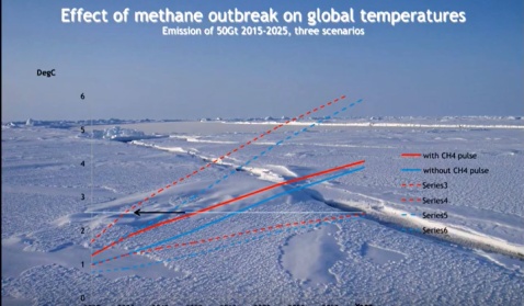
13. This increase in warming comes at a very very high cost because that model was actually an economics model, the PAGE model, and it came to some very large figure like 60 trillion dollars as the extra cost to the planet (??) over a century of methane emissions due to the retreat of sea ice. So retreat of sea ice may have economic opportunities for the world (Northwest Passsage, oil and gas exploration) but the costs are going to be very much greater because of the impact of the resulting climate change on the planet as a whole. (??).

PART 2: CRITICAL COMMENTARY ON THE CLAIMS MADE IN THE LECTURE

1. A PLANETARY SCOPE FOR THE IMPACTS OF ARCTIC SEA ICE MELT: In three different instances, a claim is made for a planetary scope and relevance of climate change and Arctic sea ice melt in terms of the implications for of an ice free Arctic and its dire and costly impacts. It is claimed that (1)“the current retreat of sea ice has implications for the climate and for the future of our planet, (2) “This increase in warming comes at a very very high cost, a very large figure like 60 trillion dollars as the extra cost to the planet” (3) “So retreat of sea ice may have economic opportunities for the world but the costs are going to be very much greater because of the impact of the resulting climate change on the planet as a whole“.
2. Kindly consider that 99.7% of the planet has no economy, no climate,  no sea, no Arctic, and no sea ice. The crust of the planet consisting of land and ocean where we live and where we have things like climate, climate change, Arctic sea ice, and climate scientists, composes not more than 0.3% of the planet. Surface phenomena observed on the crust of the planet by climate scientists, such as climate change, sea ice melt, albedo loss, feedback warming, sea level rise, and economics are peculiar to the crust and have no relevance to the the rest of the planet from the lithosphere down to the mantle and the core that compose 99.7% of the planet. No matter how great the horror of fossil fuel emissions and climate change, it is not possible to represent AGW in a planetary context.
3. THE FAILED ICE-FREE ARCTIC OBSESSION OF CLIMATE SCIENCE: At least since 1999, climate science has been seized by the obsession with an ice free Arctic and its claimed feedback and planetary horrors as the scientific substance of the case against fossil fuels. This effort has been a dismal and comical failure as seen in the list of failed claims to an imminent ice free Arctic that appears at the end of this section. These failures have convinced some climate activists to abandon the idea altogether and simply paint the horror of an ice free Arctic based on a hypothetical event [LINK] .
4. STEEP DECLINE IN SEPTEMBER MINIMUM SEA ICE VOLUME: It is shown in paragraph#7 of PART-1 that Arctic September Minimum Sea Ice Volume (ASMSIV) had undergone a dramatic decline from 1979 to 2011. This decline is then attributed to AGW climate change without any information as to how his causation was determined. Such attribution is arbitrary and it contains no causation information.
5. In terms of correlation analysis, one method of providing evidence of causation, that global warming causes the decline in ASMSIV, is to show that ASMSIV is responsive to AGW temperature. Such responsiveness should be apparent in the detrended correlation between surface temperature and ASMSIV at the appropriate time scale for the causation.
6. This analysis is presented in a related post [LINK] for ASMSIV data from 1979 to 2019 against UAH lower troposphere temperature over the North Polar region for the same period. No detrended correlation is found at an annual time scale to support the assumption by the lecturer that year to year changes in  ASMSIV can be explained by year to year changes in AGW temperature. Therefore, there is no evidence that changes in ASMSIV can be explained in terms of AGW. 
7. It is likely that the strange combination of obsession and frustration of climate science with ASMSIV  derives from their atmosphere bias such that all observed changes are explained in terms of atmospheric CO2 and fossil fuel emissions and that therefore a possible role of the geology of the Arctic in Arctic phenomena having to do with ocean temperature and ice melt are overlooked. 
8. The Arctic is geologically active. A survey of its geological features is presented in a related post [LINK] . Specific features of Arctic geology that apply to Svalbard and to the Chukchi Sea are listed separately [LINK] [LINK] .
9. These geological features of the Arctic do not constitute evidence or proof that geological forces cause ASMSIV but their presence implies that these forces must be considered in the analysis particularly since climate science has simply assumed that ASMSIV is driven by AGW without proof or evidence. The case against fossil fuel emissions is not clear but murky and sinister.
10. THE 60 TRILLION DOLLAR PRICE TAG OF ASMSIV:  The PAGE model of the economic cost of AGW was used to estimate the cost “to the planet” of AGW driven ASMSIV if it were to cause methane release from known methane hydrate deposits on the continental shelf. An estimate of 50 gigatonnes of methane release was used. The PAGE model estimated that the the impact of the methane on AGW would add another $60 trillion to the global cost of AGW. This enormous cost is thus claimed to outweigh any economic gains to be had from an ice free Arctic in terms of shipping through the Northwest Passage and oil and gas exploration. It also stands as the cost of failure to take climate action at much lower cost to prevent the horror of the ASMSIV from happening. This is a kind of Mafia tactic to extract climate action and to downplay the economic advantages of ASMSIV. Yet, without evidence to relate fossil fuel emissions to ASMSIV it cannot be claimed that climate action will have the assumed effect of moderating what is being presented as an explosive, dangerous, and costly crisis. 
11. As things stand, no causation is established for the sharp downward trend in ASMSIV seen in the chart in paragraph#7 of the lecture. Therefore,  no claim can be made that climate action will moderate the ASMSIV trend such that the budget for such action must be weighed against a $60 trillion cost of inaction estimated by economists. 

1. FAILED ICE FREE ARCTIC FORECASTS: 1999, STUDY SHOWS ARCTIC ICE SHRINKING BECAUSE OF GLOBAL WARMING. Sea ice in the Arctic Basin is shrinking by 14000 square miles per year because of global warming caused by human activity according to a new international study that used 46 years of data and sophisticated computer simulation models to tackle the specific question of whether the loss of Arctic ice is a natural variation or caused by global warming. The computer model says that the probability that these changes were caused by natural variation is 1% but when global warming was added to the model the ice melt was a perfect fit. Therefore the ice melt is caused by human activities that emit greenhouse gases.
2. 2003, SOOT WORSE FOR GLOBAL WARMING THAN PREVIOUSLY THOUGHT
   Soot that lands on snow has caused ¼ of the warming since 1880 because dirty snow traps more solar heat than pristine snow and induces a strong warming effect, according to a new computer model by James Hansen of NASA. It explains why sea ice and glaciers are melting faster than they should. Reducing soot emissions is an effective tool to curb global warming. It is easier to cut soot emissions than it is to cut CO2 emissions but we still need to reduce CO2 emissions in order to stabilize the atmosphere.
3. 2004, ARCTIC CLIMATE IMPACT ASSESSMENT
   An unprecedented 4-year study of the Arctic shows that polar bears, walruses, and some seals are becoming extinct. Arctic summer sea ice may disappear entirely. Combined with a rapidly melting Greenland ice sheet, it will raise the sea level 3 feet by 2100 inundating lowlands from Florida to Bangladesh. Average winter temperatures in Alaska and the rest of the Arctic are projected to rise an additional 7 to 13 degrees over the next 100 years because of increasing emissions of greenhouse gases from human activities. The area is warming twice as fast as anywhere else because of global air circulation patterns and natural feedback loops, such as less ice reflecting sunlight, leading to increased warming at ground level and more ice melt. Native peoples’ ways of life are threatened. Animal migration patterns have changed, and the thin sea ice and thawing tundra make it too dangerous for humans to hunt and travel.
4. 2004, RAPID ARCTIC WARMING BRINGS SEA LEVEL RISE
   The Arctic Climate Impact Assessment (ACIA) report says: increasing greenhouse gases from human activities is causing the Arctic to warm twice as fast as the rest of the planet; in Alaska, western Canada, and eastern Russia winter temperatures have risen by 2C to 4C in the last 50 years; the Arctic will warm by 4C to 7C by 2100. A portion of Greenland’s ice sheet will melt; global sea levels will rise; global warming will intensify. Greenland contains enough melting ice to raise sea levels by 7 meters; Bangkok, Manila, Dhaka, Florida, Louisiana, and New Jersey are at risk of inundation; thawing permafrost and rising seas threaten Arctic coastal regions; climate change will accelerate and bring about profound ecological and social changes; the Arctic is experiencing the most rapid and severe climate change on earth and it’s going to get a lot worse; Arctic summer sea ice will decline by 50% to 100%; polar bears will be driven towards extinction; this report is an urgent SOS for the Arctic; forest fires and insect infestations will increase in frequency and intensity; changing vegetation and rising sea levels will shrink the tundra to its lowest level in 21000 years; vanishing breeding areas for birds and grazing areas for animals will cause extinctions of many species; “if we limit emission of heat trapping carbon dioxide we can still help protect the Arctic and slow global warming”.
5. 2007: THE ARCTIC IS SCREAMING. Climate science declares that the low sea ice extent in the Arctic is the leading indicator of climate change. We are told that the Arctic “is screaming”, that Arctic sea ice extent is the “canary in the coal mine”, and that Polar Bears and other creatures in the Arctic are dying off and facing imminent extinction. Scientists say that the melting sea ice has set up a positive feedback system that would cause the summer melts in subsequent years to be greater and greater until the Arctic becomes ice free in the summer of 2012. We must take action immediately to cut carbon dioxide emissions from fossil fuels. [DETAILS] 
6. 2007: THE ICE FREE ARCTIC CLAIMS GAIN MOMENTUM: The unusual summer melt of Arctic sea ice in 2007 has encouraged climate science to warn the world that global warming will cause a steep decline in the amount of ice left in subsequent summer melts until the Arctic becomes ice free in summer and that could happen as soon as 2080 or maybe 2060 or it could even be 2030. This time table got shorter and shorter until, without a “scientific” explanation, the ice free year was brought up to 2013. In the meantime, the data showed that in 2008 and 2009 the summer melt did not progressively increase as predicted but did just the opposite by making a comeback in 2008 that got even stronger in 2009. [DETAILS]
7. 2008: POSITIVE FEEDBACK: ARCTIC SEA ICE IN A DOWNWARD SPIRAL
   Our use of fossil fuels is devastating the Arctic where the volume of sea ice “fell to its lowest recorded level to date” this year and that reduced ice coverage is causing a non-linear acceleration in the loss of polar ice because there is less ice to reflect sunlight. [DETAILS]
8. 2008: THE ARCTIC WILL BE ICE FREE IN SUMMER IN 2008, 2013, 2030, OR 2100. The unusually low summer sea ice extent in the Arctic in 2007
   The IPCC has taken note and has revised its projection of an ice free Arctic first from 2008 to 2013 and then again from 2013 to 2030. The way things are going it may be revised again to the year 2100. [DETAILS]
9. 2008: THE POLAR BEAR IS THREATENED BY OUR USE OF FOSSIL FUELS
   The survival of the polar bear is threatened because man made global warming is melting ice in the Arctic. It is true that the Arctic sea ice extent was down in negative territory in September 2007. This event emboldened global warming scaremongers to declare it a climate change disaster caused by greenhouse gas emissions from fossil fuels and to issue a series of scenarios about environmental holocaust yet to come. [DETAILS]
10. 2009: SUMMER ARCTIC SEA ICE EXTENT IN 2009 THE 3RD LOWEST ON RECORD: The second lowest was 2008 and the first lowest was 2007. This is not a trend that shows that things are getting worse. It shows that things are getting better and yet it is being sold and being bought as evidence that things are getting worse due to rising fossil fuel emissions. [DETAILS]
11. 2009: THE ARCTIC WILL BE ICE FREE IN SUMMER BY 2029
    An alarm is raised that the extreme summer melt of Arctic sea ice in 2007 was caused by humans using fossil fuels and it portends that in 20 years human caused global warming will leave the Arctic Ocean ice-free in the summer raising sea levels and harming wildlife. [DETAILS]
12. 2009: THE ARCTIC WILL BE ICE FREE IN SUMMER BY THE YEAR 2012
    Climate scientists continue to extrapolate the extreme summer melt of Arctic sea ice in 2007 to claim that the summer melt of 2007 was a climate change event and that it implies that the Arctic will be ice free in the summer from 2012 onwards. This is a devastating effect on the planet and our use of fossil fuels is to blame. [DETAILS]
13. 2009: THE SUMMER SEA ICE EXTENT IN THE ARCTIC WILL BE GONE
    Summer melt of Arctic ice was the third most extensive on record in 2009, second 2008, and the most extensive in 2007. These data show that warming due to our carbon dioxide emissions are causing summer Arctic ice to gradually diminish until it will be gone altogether. [DETAILS]

[LINK TO THE HOME PAGE OF THIS SITE]

RELATED AGW POST ON ETCW: [LINK] 

RELATED POST ON OZONE DEPLETION: [LINK]

THIS POST IS A BIBLIOGRAPHY ON THE UNRESOLVED EARLY TWENTIETH CENTURY WARMING (ETCW)  & OTHER 20TH CENTURY WARMING ISSUES

EARLY TWENTIETH CENTURY WARMING BIBLIOGRAPHY

1. Delworth, Thomas L., and Thomas R. Knutson. “Simulation of early 20th century global warming.” Science 287.5461 (2000): 2246-2250.  The observed global warming of the past century occurred primarily in two distinct 20-year periods, from 1925 to 1944 and from 1978 to the present. Although the latter warming is often attributed to a human-induced increase of greenhouse gases, causes of the earlier warming are less clear because this period precedes the time of strongest increases in human-induced greenhouse gas (radiative) forcing. Results from a set of six integrations of a coupled ocean-atmosphere climate model suggest that the warming of the early 20th century could have resulted from a combination of human-induced radiative forcing and an unusually large realization of internal multidecadal variability of the coupled ocean-atmosphere system. This conclusion is dependent on the model’s climate sensitivity, internal variability, and the specification of the time-varying human-induced radiative forcing.
2. Brönnimann, Stefan. “Early twentieth-century warming.” Nature Geoscience 2.11 (2009): 735-736.  The most pronounced warming in the historical global climate record prior to the recent warming occurred over the first half of the 20th century and is known as the Early Twentieth Century Warming (ETCW). Understanding this period and the subsequent slowdown of warming is key to disentangling the relationship between decadal variability and the response to human influences in the present and future climate. This review discusses the observed changes during the ETCW and hypotheses for the underlying causes and mechanisms. Attribution studies estimate that about a half (40–54%; p > .8) of the global warming from 1901 to 1950 was forced by a combination of increasing greenhouse gases and natural forcing, offset to some extent by aerosols. Natural variability also made a large contribution, particularly to regional anomalies like the Arctic warming in the 1920s and 1930s. The ETCW period also encompassed exceptional events, several of which are touched upon: Indian monsoon failures during the turn of the century, the “Dust Bowl” droughts and extreme heat waves in North America in the 1930s, the World War II period drought in Australia between 1937 and 1945; and the European droughts and heat waves of the late 1940s and early 1950s. Understanding the mechanisms involved in these events, and their links to large scale forcing is an important test for our understanding of modern climate change and for predicting impacts of future change. This article is categorized under: • Paleoclimates and Current Trends > Modern Climate Change
3. Cowan, Tim, et al. “Factors contributing to record-breaking heat waves over the Great Plains during the 1930s Dust Bowl.” Journal of Climate 30.7 (2017): 2437-2461.  Record-breaking summer heat waves were experienced across the contiguous United States during the decade-long “Dust Bowl” drought in the 1930s. Using high-quality daily temperature observations, the Dust Bowl heat wave characteristics are assessed with metrics that describe variations in heat wave activity and intensity. Despite the sparser station coverage in the early record, there is robust evidence for the emergence of exceptional heat waves across the central Great Plains, the most extreme of which were preconditioned by anomalously dry springs. This is consistent with the entire twentieth-century record: summer heat waves over the Great Plains develop on average ~15–20 days earlier after anomalously dry springs, compared to summers following wet springs. Heat waves following dry springs are also significantly longer and hotter, indicative of the importance of land surface feedbacks in heat wave intensification. A distinctive anomalous continental-wide circulation pattern accompanied exceptional heat waves in the Great Plains, including those of the Dust Bowl decade. An anomalous broad surface pressure ridge straddling an upper-level blocking anticyclone over the western United States forced substantial subsidence and adiabatic warming over the Great Plains, and triggered anomalous southward warm advection over southern regions. This prolonged and amplified the heat waves over the central United States, which in turn gradually spread westward following heat wave emergence. The results imply that exceptional heat waves are preconditioned, triggered, and strengthened across the Great Plains through a combination of spring drought, upper-level continental-wide anticyclonic flow, and warm advection from the north.
4. Wegmann, Martin, Stefan Brönnimann, and Gilbert P. Compo. “Tropospheric circulation during the early twentieth century Arctic warming.” Climate dynamics 48.7-8 (2017): 2405-2418.  The early twentieth century Arctic warming (ETCAW) between 1920 and 1940 is an exceptional feature of climate variability in the last century. Its warming rate was only recently matched by recent warming in the region. Unlike recent warming largely attributable to anthropogenic radiative forcing, atmospheric warming during the ETCAW was strongest in the mid-troposphere and is believed to be triggered by an exceptional case of natural climate variability. Nevertheless, ultimate mechanisms and causes for the ETCAW are still under discussion. Here we use state of the art multi-member global circulation models, reanalysis and reconstruction datasets to investigate the internal atmospheric dynamics of the ETCAW. We investigate the role of boreal winter mid-tropospheric heat transport and circulation in providing the energy for the large scale warming. Analyzing sensible heat flux components and regional differences, climate models are not able to reproduce the heat flux evolution found in reanalysis and reconstruction datasets. These datasets show an increase of stationary eddy heat flux and a decrease of transient eddy heat flux during the ETCAW. Moreover, tropospheric circulation analysis reveals the important role of both the Atlantic and the Pacific sectors in the convergence of southerly air masses into the Arctic during the warming event. Subsequently, it is suggested that the internal dynamics of the atmosphere played a major role in the formation in the ETCAW.
5. Stolpe, Martin B., Iselin Medhaug, and Reto Knutti. “Contribution of Atlantic and Pacific multidecadal variability to twentieth-century temperature changes.” Journal of Climate 30.16 (2017): 6279-6295.  Recent studies have suggested that significant parts of the observed warming in the early and the late twentieth century were caused by multidecadal internal variability centered in the Atlantic and Pacific Oceans. Here, a novel approach is used that searches for segments of unforced preindustrial control simulations from global climate models that best match the observed Atlantic and Pacific multidecadal variability (AMV and PMV, respectively). In this way, estimates of the influence of AMV and PMV on global temperature that are consistent both spatially and across variables are made. Combined Atlantic and Pacific internal variability impacts the global surface temperatures by up to 0.15°C from peak-to-peak on multidecadal time scales. Internal variability contributed to the warming between the 1920s and 1940s, the subsequent cooling period, and the warming since then. However, variations in the rate of warming still remain after removing the influence of internal variability associated with AMV and PMV on the global temperatures. During most of the twentieth century, AMV dominates over PMV for the multidecadal internal variability imprint on global and Northern Hemisphere temperatures. Less than 10% of the observed global warming during the second half of the twentieth century is caused by internal variability in these two ocean basins, reinforcing the attribution of most of the observed warming to anthropogenic forcings.
6. Tokinaga, Hiroki, Shang-Ping Xie, and Hitoshi Mukougawa. “Early 20th-century Arctic warming intensified by Pacific and Atlantic multidecadal variability.” Proceedings of the National Academy of Sciences 114.24 (2017): 6227-6232.  With amplified warming and record sea ice loss, the Arctic is the canary of global warming. The historical Arctic warming is poorly understood, limiting our confidence in model projections. Specifically, Arctic surface air temperature increased rapidly over the early 20th century, at rates comparable to those of recent decades despite much weaker greenhouse gas forcing. Here, we show that the concurrent phase shift of Pacific and Atlantic interdecadal variability modes is the major driver for the rapid early 20th-century Arctic warming. Atmospheric model simulations successfully reproduce the early Arctic warming when the interdecadal variability of sea surface temperature (SST) is properly prescribed. The early 20th-century Arctic warming is associated with positive SST anomalies over the tropical and North Atlantic and a Pacific SST pattern reminiscent of the positive phase of the Pacific decadal oscillation. Atmospheric circulation changes are important for the early 20th-century Arctic warming. The equatorial Pacific warming deepens the Aleutian low, advecting warm air into the North American Arctic. The extratropical North Atlantic and North Pacific SST warming strengthens surface westerly winds over northern Eurasia, intensifying the warming there. Coupled ocean–atmosphere simulations support the constructive intensification of Arctic warming by a concurrent, negative-to-positive phase shift of the Pacific and Atlantic interdecadal modes. Our results aid attributing the historical Arctic warming and thereby constrain the amplified warming projected for this important region.
7. Hegerl, Gabriele C., et al. “The early 20th century warming: anomalies, causes, and consequences.” Wiley Interdisciplinary Reviews: Climate Change 9.4 (2018): e522.  The most pronounced warming in the historical global climate record prior to the recent warming occurred over the first half of the 20th century and is known as the Early Twentieth Century Warming (ETCW). Understanding this period and the subsequent slowdown of warming is key to disentangling the relationship between decadal variability and the response to human influences in the present and future climate. This review discusses the observed changes during the ETCW and hypotheses for the underlying causes and mechanisms. Attribution studies estimate that about a half (40–54%; p > .8) of the global warming from 1901 to 1950 was forced by a combination of increasing greenhouse gases and natural forcing, offset to some extent by aerosols. Natural variability also made a large contribution, particularly to regional anomalies like the Arctic warming in the 1920s and 1930s. The ETCW period also encompassed exceptional events, several of which are touched upon: Indian monsoon failures during the turn of the century, the “Dust Bowl” droughts and extreme heat waves in North America in the 1930s, the World War II period drought in Australia between 1937 and 1945; and the European droughts and heat waves of the late 1940s and early 1950s. Understanding the mechanisms involved in these events, and their links to large scale forcing is an important test for our understanding of modern climate change and for predicting impacts of future change.
8. Butler, James H., et al. “A record of atmospheric halocarbons during the twentieth century from polar firn air.” Nature 399.6738 (1999): 749-755.  Measurements of trace gases in air trapped in polar firn (unconsolidated snow) demonstrate that natural sources of chlorofluorocarbons, halons, persistent chlorocarbon solvents and sulphur hexafluoride to the atmosphere are minimal or non-existent. Atmospheric concentrations of these gases, reconstructed back to the late nineteenth century, are consistent with atmospheric histories derived from anthropogenic emission rates and known atmospheric lifetimes. The measurements confirm the predominance of human activity in the atmospheric budget of organic chlorine, and allow the estimation of atmospheric histories of halogenated gases of combined anthropogenic and natural origin. The pre-twentieth-century burden of methyl chloride was close to that at present, while the burden of methyl bromide was probably over half of today’s value.
9. Tett, Simon FB, et al. “Estimation of natural and anthropogenic contributions to twentieth century temperature change.” Journal of Geophysical Research: Atmospheres 107.D16 (2002): ACL-10.  Using a coupled atmosphere/ocean general circulation model, we have simulated the climatic response to natural and anthropogenic forcings from 1860 to 1997. The model, HadCM3, requires no flux adjustment and has an interactive sulphur cycle, a simple parameterization of the effect of aerosols on cloud albedo (first indirect effect), and a radiation scheme that allows explicit representation of well‐mixed greenhouse gases. Simulations were carried out in which the model was forced with changes in natural forcings (solar irradiance and stratospheric aerosol due to explosive volcanic eruptions), well‐mixed greenhouse gases alone, tropospheric anthropogenic forcings (tropospheric ozone, well‐mixed greenhouse gases, and the direct and first indirect effects of sulphate aerosol), and anthropogenic forcings (tropospheric anthropogenic forcings and stratospheric ozone decline). Using an “optimal detection” methodology to examine temperature changes near the surface and throughout the free atmosphere, we find that we can detect the effects of changes in well‐mixed greenhouse gases, other anthropogenic forcings (mainly the effects of sulphate aerosols on cloud albedo), and natural forcings. Thus these have all had a significant impact on temperature. We estimate the linear trend in global mean near‐surface temperature from well‐mixed greenhouse gases to be 0.9 ± 0.24 K/century, offset by cooling from other anthropogenic forcings of 0.4 ± 0.26 K/century, giving a total anthropogenic warming trend of 0.5 ± 0.15 K/century. Over the entire century, natural forcings give a linear trend close to zero. We found no evidence that simulated changes in near‐surface temperature due to anthropogenic forcings were in error. However, the simulated tropospheric response, since the 1960s, is ∼50% too large. Our analysis suggests that the early twentieth century warming can best be explained by a combination of warming due to increases in greenhouse gases and natural forcing, some cooling due to other anthropogenic forcings, and a substantial, but not implausible, contribution from internal variability. In the second half of the century we find that the warming is largely caused by changes in greenhouse gases, with changes in sulphates and, perhaps, volcanic aerosol offsetting approximately one third of the warming. Warming in the troposphere, since the 1960s, is probably mainly due to anthropogenic forcings, with a negligible contribution from natural forcings.
10. Thompson, David WJ, et al. “Signatures of the Antarctic ozone hole in Southern Hemisphere surface climate change.” Nature Geoscience 4.11 (2011): 741-749.  Anthropogenic emissions of carbon dioxide and other greenhouse gases have driven and will continue to drive widespread climate change at the Earth’s surface. But surface climate change is not limited to the effects of increasing atmospheric greenhouse gas concentrations. Anthropogenic emissions of ozone-depleting gases also lead to marked changes in surface climate, through the radiative and dynamical effects of the Antarctic ozone hole. The influence of the Antarctic ozone hole on surface climate is most pronounced during the austral summer season and strongly resembles the most prominent pattern of large-scale Southern Hemisphere climate variability, the Southern Annular Mode. The influence of the ozone hole on the Southern Annular Mode has led to a range of significant summertime surface climate changes not only over Antarctica and the Southern Ocean, but also over New Zealand, Patagonia and southern regions of Australia. Surface climate change as far equatorward as the subtropical Southern Hemisphere may have also been affected by the ozone hole. Over the next few decades, recovery of the ozone hole and increases in greenhouse gases are expected to have significant but opposing effects on the Southern Annular Mode and its attendant climate impacts during summer.
11. Compo, Gilbert P., et al. “The twentieth century reanalysis project.” Quarterly Journal of the Royal Meteorological Society 137.654 (2011): 1-28. The Twentieth Century Reanalysis (20CR) project is an international effort to produce a comprehensive global atmospheric circulation dataset spanning the twentieth century, assimilating only surface pressure reports and using observed monthly sea‐surface temperature and sea‐ice distributions as boundary conditions. It is chiefly motivated by a need to provide an observational dataset with quantified uncertainties for validations of climate model simulations of the twentieth century on all time‐scales, with emphasis on the statistics of daily weather. It uses an Ensemble Kalman Filter data assimilation method with background ‘first guess’ fields supplied by an ensemble of forecasts from a global numerical weather prediction model. This directly yields a global analysis every 6 hours as the most likely state of the atmosphere, and also an uncertainty estimate of that analysis.The 20CR dataset provides the first estimates of global tropospheric variability, and of the dataset’s time‐varying quality, from 1871 to the present at 6‐hourly temporal and 2° spatial resolutions. Comparisons with independent radiosonde data indicate that the reanalyses are generally of high quality. The quality in the extratropical Northern Hemisphere throughout the century is similar to that of current three‐day operational NWP forecasts. Intercomparisons over the second half‐century of these surface‐based reanalyses with other reanalyses that also make use of upper‐air and satellite data are equally encouraging. It is anticipated that the 20CR dataset will be a valuable resource to the climate research community for both model validations and diagnostic studies. Some surprising results are already evident. For instance, the long‐term trends of indices representing the North Atlantic Oscillation, the tropical Pacific Walker Circulation, and the Pacific–North American pattern are weak or non‐existent over the full period of record. The long‐term trends of zonally averaged precipitation minus evaporation also differ in character from those in climate model simulations of the twentieth century.
12. Smith, Karen L., Lorenzo M. Polvani, and Daniel R. Marsh. “Mitigation of 21st century Antarctic sea ice loss by stratospheric ozone recovery.” Geophysical Research Letters 39.20 (2012).  We investigate the effect of stratospheric ozone recovery on Antarctic sea ice in the next half‐century, by comparing two ensembles of integrations of the Whole Atmosphere Community Climate Model, from 2001 to 2065. One ensemble is performed by specifying all forcings as per the Representative Concentration Pathway 4.5; the second ensemble is identical in all respects, except for the surface concentrations of ozone depleting substances, which are held fixed at year 2000 levels, thus preventing stratospheric ozone recovery. Sea ice extent declines in both ensembles, as a consequence of increasing greenhouse gas concentrations. However, we find that sea ice loss is ∼33% greater for the ensemble in which stratospheric ozone recovery does not take place, and that this effect is statistically significant. Our results, which confirm a previous study dealing with ozone depletion, suggest that ozone recovery will substantially mitigate Antarctic sea ice loss in the coming decades.
13. Egorova, Tatiana, et al. “Contributions of natural and anthropogenic forcing agents to the early 20th century warming.” Frontiers in Earth Science 6 (2018): 206.  The warming observed in the early 20th century (1910–1940) is one of the most intriguing and least understood climate anomalies of the 20th century. To investigate the contributions of natural and anthropogenic factors to changes in the surface temperature, we performed seven model experiments using the chemistry-climate model with interactive ocean SOCOL3-MPIOM. Contributions of energetic particle precipitation, heavily (shortwave UV) and weakly (longwave UV, visible, and infrared) absorbed solar irradiances, well-mixed greenhouse gases (WMGHGs), tropospheric ozone precursors, and volcanic eruptions were considered separately. Model results suggest only about 0.3 K of global and annual mean warming during the considered 1910–1940 period, which is smaller than the trend obtained from observations by about 25%. We found that half of the simulated global warming is caused by the increase of WMGHGs (CO₂, CH₄, and N₂O), while the increase of the weakly absorbed solar irradiance is responsible for approximately one third of the total warming. Because the behavior of WMGHGs is well constrained, only higher solar forcing or the inclusion of new forcing mechanisms can help to reach better agreement with observations. The other forcing agents considered (heavily absorbed UV, energetic particles, volcanic eruptions, and tropospheric ozone precursors) contribute less than 20% to the annual and global mean warming; however, they can be important on regional/seasonal scales.
14. Polvani, Lorenzo M., et al. “Significant weakening of Brewer‐Dobson circulation trends over the 21st century as a consequence of the Montreal Protocol.” Geophysical Research Letters 45.1 (2018): 401-409.  It is well established that increasing greenhouse gases, notably CO₂, will cause an acceleration of the stratospheric Brewer‐Dobson circulation (BDC) by the end of this century. We here present compelling new evidence that ozone depleting substances are also key drivers of BDC trends. We do so by analyzing and contrasting small ensembles of “single‐forcing” integrations with a stratosphere resolving atmospheric model with interactive chemistry, coupled to fully interactive ocean, land, and sea ice components. First, confirming previous work, we show that increasing concentrations of ozone depleting substances have contributed a large fraction of the BDC trends in the late twentieth century. Second, we show that the phasing out of ozone depleting substances in coming decades—as a consequence of the Montreal Protocol—will cause a considerable reduction in BDC trends until the ozone hole is completely healed, toward the end of the 21st century.
15. Polvani, Lorenzo M., and Katinka Bellomo. “The Key Role of Ozone-Depleting Substances in Weakening the Walker Circulation in the Second Half of the Twentieth Century.” Journal of Climate 32.5 (2019): 1411-1418.  It is widely appreciated that ozone-depleting substances (ODS), which have led to the formation of the Antarctic ozone hole, are also powerful greenhouse gases. In this study, we explore the consequence of the surface warming caused by ODS in the second half of the twentieth century over the Indo-Pacific Ocean, using the Whole Atmosphere Chemistry Climate Model (version 4). By contrasting two ensembles of chemistry–climate model integrations (with and without ODS forcing) over the period 1955–2005, we show that the additional greenhouse effect of ODS is crucial to producing a statistically significant weakening of the Walker circulation in our model over that period. When ODS concentrations are held fixed at 1955 levels, the forcing of the other well-mixed greenhouse gases alone leads to a strengthening—rather than weakening—of the Walker circulation because their warming effect is not sufficiently strong. Without increasing ODS, a surface warming delay in the eastern tropical Pacific Ocean leads to an increase in the sea surface temperature gradient between the eastern and western Pacific, with an associated strengthening of the Walker circulation. When increasing ODS are added, the considerably larger total radiative forcing produces a much faster warming in the eastern Pacific, causing the sign of the trend to reverse and the Walker circulation to weaken. Our modeling result suggests that ODS may have been key players in the observed weakening of the Walker circulation over the second half of the twentieth century.
16. Abalos, Marta, et al. “New Insights on the Impact of Ozone‐Depleting Substances on the Brewer‐Dobson Circulation.” Journal of Geophysical Research: Atmospheres 124.5 (2019): 2435-2451.  It has recently been recognized that, in addition to greenhouse gases, anthropogenic emissions of ozone‐depleting substances (ODS) can induce long‐term trends in the Brewer‐Dobson circulation (BDC). Several studies have shown that a substantial fraction of the residual circulation acceleration over the last decades of the twentieth century can be attributed to increasing ODS. Here the mechanisms of this influence are examined, comparing model runs to reanalysis data and evaluating separately the residual circulation and mixing contributions to the mean age of air trends. The effects of ozone depletion in the Antarctic lower stratosphere are found to dominate the ODS impact on the BDC, while the direct radiative impact of these substances is negligible over the period of study. We find qualitative agreement in austral summer BDC trends between model and reanalysis data and show that ODS are the main driver of both residual circulation and isentropic mixing trends over the last decades of the twentieth century. Moreover, aging by isentropic mixing is shown to play a key role on ODS‐driven age of air trends.
17. Polvani, L. M., et al. “Substantial twentieth-century Arctic warming caused by ozone-depleting substances.” Nature Climate Change (2020): 1-4.  The rapid warming of the Arctic, perhaps the most striking evidence of climate change, is believed to have arisen from increases in atmospheric concentrations of GHG since the Industrial Revolution. While the dominant role of carbon dioxide is undisputed, another important set of anthropogenic GHGs was also being emitted over the second half of the twentieth century: ozone depleting substances (ODS). These compounds, in addition to causing the ozone hole over Antarctica, have long been recognized as powerful GHG. However, their contribution to Arctic warming has not been quantified. We do so here by analysing ensembles of climate model integrations specifically designed for this purpose, spanning the period 1955–2005 when atmospheric concentrations of ODS increased rapidly. We show that, when ODS are kept fixed, forced Arctic surface warming and forced sea-ice loss are only half as large as when ODS are allowed to increase. We also demonstrate that the large impact of ODS on the Arctic occurs primarily via direct radiative warming, not via ozone depletion. Our findings reveal a substantial contribution of ODS to recent Arctic warming, and highlight the importance of the Montreal Protocol as a major climate change-mitigation treaty.

THIS POST IS A CRITICAL EVALUATION OF A TED TALK ON OCEAN ACIDIFICATION BY TRIONA MCGRATH   . THE TRANSCRIPT OF THE TALK IS PRESENTED IN PART-1 OF THE POST WITH A CRITICAL COMMENTARY ON THE PRESENTATION IN PART-2. 

[LIST OF POSTS ON THIS SITE]

OTHER POSTS ON OCEAN ACIDIFICATION [LINK] [LINK] [LINK] [LINK] [LINK] 

PART-1: TRANSCRIPT OF THE TED TALK BY TRIONA MCGRATH 

[LINK TO YOUTUBE VIDEO] 

1. Do you ever think about how important the oceans are in our daily lives? The oceans cover 2/3 of the planet. They provide half the oxygen we breathe. They moderate our climate. And they provide dogs (drugs?) and medicine, and food including 20% protein to feed the entire world population.
2. People used to think that the oceans are so vast that they wouldn’t be affected by human activities. Well today I am going to tell you about a serious reality that is changing our oceans. It’s called ocean acidification or the evil twin of climate change. Did you know that the oceans have absorbed 25% of all of the CO2 that we have emitted into the atmosphere?
3. Now this is just another great service provided by the oceans since carbon dioxide is one of the greenhouse gases that’s causing climate change. But as we keep pumping more and more and more carbon dioxide into the atmosphere, more is dissolving into the oceans and this is what’s changing our ocean chemistry. When carbon dioxide dissolves in seawater it undergoes a number of chemical reactions. Now lucky for you I don’t have time to get into the details of the chemistry for today. But I will tell you that as more carbon dioxide enters the ocean, the seawater pH goes down and that basically means that there is an increase in ocean acidity.
4. And this whole process is called ocean acidification and it is happening alongside climate change. Scientists have been monitoring ocean acidification for over two decades. This figure is an important time series in Hawaii and the top line shows a steadily increasing concentration of carbon dioxide in the atmosphere; and this is directly as a result of human activities. The line underneath shows the increasing concentrations of carbon dioxide that is dissolved in the surface of the ocean which you can see is increasing at the same rate as carbon dioxide in the atmosphere since measurements began. The line in the bottom then shows the change in chemistry. As more carbon dioxide has entered the ocean, the seawater pH has gone down, which basically means that there has been an increase in ocean acidity.
5. Now in Ireland, scientists are also monitoring ocean acidification, Scientific and Marine Institute and NUI Galway (National University of Ireland at Galway). And we too are seeing acidification at the same rate as the main ocean time series sites around the world. So it’s happening right at our doorstep. Now I’d like to give you an example of just how we collect our data to monitor a changing ocean. Firstly, we collect a lot of our samples in the middle pf winter so as you can imagine in the North Atlantic we got hit with some seriously stormy conditions so we got hit with some motion sickness but we did collect some very valuable data. So we lower the instruments over the side of the ship and there are sensors that are mounted on the bottom that can tell us information about the surrounding water. Such as temperature, or dissolved oxygen; and we can collect our sea water samples in these large bottles. So we start at the bottom which can be over 4 km deep (4000 meters or 13,123 feet), just off our continental shelf; and we take samples at regular intervals right up to the surface. We take the sea-water back on the deck and then we can either analyze them on the ship or back in the laboratory so the different chemical parameters.
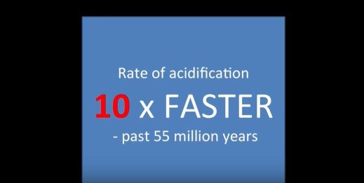
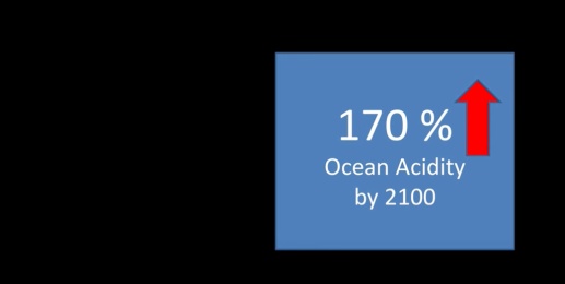
6. But why should we care? How is ocean acidification going to affect all of us? Well, here are the worrying facts. There has already been an increase in ocean acidity of 26% since pre-industrial times which is directly due to human activities. Unless we can start slowing down our carbon dioxide emissions, we are expecting an increase in ocean acidity of 170% by the end of this century. I mean this is within our children’s lifetime. This rate of acidification is ten times faster than any acidification in our oceans for over 55 million years. So our marine life has never ever experienced such a fast rate of change before. So we literally could not know how they’re going to cope. 
7. Now there was a natural acidification event millions of years ago which was much slower than what we are seeing today and this coincided with a mass extinction of many marine species. So is that what we’re headed for? Well, maybe! Studies are showing that while some species are actually doing quite well, but many are showing a negative response. This is one of the big concerns as ocean acidification increases, the concentration of carbonate ions in seawater decreased. Now these ions are basically the building blocks for many marine species to make their cells. For example crabs or mussels or oysters. Another example are corals. They also need the carbonate ions in seawater to make their coral structure in order to build a coral reef. As ocean acidity increases, and the concentration of carbonate ions decreases, these species first find it more difficult to make their cells, and at even lower levels, they can actually begin to dissolve.
8. Shown above is a terapod, also called a sea butterfly, and it’s an important food source in the ocean for many species – from krill to salmon right up to whales. The shell of the terapod was placed into sea water at a pH that we are expecting at the end of the century. After only 45 days at this very realistic pH, you can see that the shell has almost completely dissolved. So ocean acidification could affect right up through the food chain and right on to our dinner plates. i mean who here likes shellfish? or a salmon? or many other fish species whose food source in the ocean could be affected.
9. Shown above are cold water corals. And did you know that we actually have cold water corals in Irish waters just off our continental shelf. And they support a rich biodiversity including some very important fisheries. It is projected that by the end of this century 70% of all known cold water corals in the entire ocean will be surrounded by seawater that is dissolving their coral structure.
10. The last example I have are these healthy tropical corals. They were placed in seawater at the pH we are expecting in the year 2100. After 6 months the corals had almost completely dissolved (shown in the graphic above). Now coral reefs support 25% of all marine life in the entire ocean. All marine life! So you can see that ocean acidification is a global threat. I have an 8-month-old baby boy. Unless we start now to slow this down, I dread to think what our oceans will look like when he is a grown man.
11. We will see acidification. We have already put too much carbon dioxide into the atmosphere. But we can slow this down. We can prevent the worst case scenario. The only way of doing that is by reducing our carbon dioxide emissions. This is important for both you and I, for industry, for government. We need to work together and slow down ocean acidification. And then we can slow down global warming. Slow down ocean acidification. And help to maintain a healthy ocean and a healthy planet for our generation and for generations to come.

PART-2: CRITICAL COMMENTARY

1. As in other Ocean Acidification (OA) scenarios [LINK] [LINK] [LINK] [LINK] [LINK], OA is presented as an alarming and dangerous development in the AGW climate change context that is already evident. However, this OA presentation is very different with respect to the timing of the  horror. Quite unlike the other alarming scenarios, where the horror of ocean acidification is evident, the presentation made here contains no such statement or implication.
2. Here, the dangerous consequences of OA are placed not in the past, nor the present, but well out in the distant future 80 years from now in the year 2100. The thesis is not that that the horror of OA has arrived, nor that it is evident in the data, but that it will surely arrive by the year 2100 unless we take climate action to reduce fossil fuel emissions. It is claimed that climate action will slow down OA to the point where it will no longer be the horror it is forecast to be in the absence of climate action.
3. In this sense, this presentation appears to be a case of climate action activism against fossil fuels where the horrors of OA are used as the rationale for changing the world’s energy infrastructure away from fossil fuels. This presentation is carefully structured anti fossil fuel activism with the motivation for cutting emissions (not using fossil fuels) provided by detailed descriptions of OA horrors that lie in wait for us in the year 2100 if we continue to use fossil fuels.
4. The causal connection between the use of fossil fuels and OA is made, as in all other OA presentations, with the unsubstantiated claim that the source of the carbon dioxide causing the acidification is our use of fossil fuels because we are “pumping more and more and more carbon dioxide into the atmosphere“.
5. In a related post [LINK] it is shown that in the 60-year period 1955-2015, inorganic CO2 concentration in the ocean went up at an average rate of 0.002 MM/L (millimoles per liter) per year. Correlation analysis is presented to test whether changes in oceanic CO2 concentration is responsive to emissions at an annual time scale. The analysis failed to show such a causal relationship between emissions and changes in oceanic CO2 concentration.
6. In that same study [LINK] , in terms of ppm by weight, the CO2 concentration of the ocean had increased from 88ppm to 110ppm for a gain of 22ppm at a rate of 0.367ppm per year. During this period fossil fuel emissions increased from 7.5 gigatonnes/year of CO2 (GTY) to 36.1GTY with cumulative emissions since 1851 rising from 258 GT to 1,505 GT with a total amount contributed in this period of 1,247 GT.  If all of these emissions had gone into the ocean it would have caused an increase of 0.91 ppm of CO2 in the ocean. Therefore, the observed rise of 22pm cannot be explained in terms of fossil fuel emissions. 
7. The claim made in paragraph 4 that causation of OA by fossil fuel emissions is established because the two time series are both rising at the same rate over the same time period, is false. Such correlations do not serve as evidence of causation. For that, a time scale for the causation must be specified and the two time series must be detrended; and a statistically significant detrended correlation at the specified time scale must exist. As shown in a related post, no evidence for such causation is found in the data at an annual time scale [LINK] .
8. These results suggest that natural sources of CO2 in the ocean itself must be considered. Known geological sources of CO2 in the ocean include plate tectonics, submarine volcanism, mantle plumes, hydrothermal vents, methane hydrates, and hydrocarbon seepage and these sources must be taken into account in the study of changes in oceanic inorganic CO2 concentration. It is necessary to overcome the extreme atmosphere bias of climate science to conduct a more realistic study of changes in oceanic CO2.
9. That experiments carried out in the laboratory with high concentrations of CO2 show shells of oceanic creatures dissolving is not relevant to a demand for reducing or eliminating fossil fuel emissions until it can be shown that the observed changes in oceanic CO2 concentration are  responsive to fossil fuel emissions. The relevance of geological activity in this regard is discussed in related posts [LINK] [LINK] [LINK] . Also, if shellfish of the deep are threatened by carbon dioxide in our fossil fuel emissions, we need an explanation for why the shellfish of the deep like to hang out near hydrothermal vents. 
   

   
10. The natural ocean acidification event in the paleo record 55 million years ago to which she refers is the PETM [LINK] where the source of the CO2 was entirely geological such that the ocean had acidified itself. In light of this and other paleo records of the impact of geological carbon on the ocean and the atmosphere, climate science insists that this time around all changes must be explained in terms of human activity by way of atmospheric CO2. This bias in climate science is a serious flaw. It weakens the science credentials on which it relies and from which it tends to derive its legitimacy.
11. CONCLUSION: A convincing case is made that if the very high carbon dioxide concentrations used in the laboratory experiments were to occur in the ocean, oceanic creatures would become grossly affected in terms of dissolving shells and other horrors. However, no matter how horrible, these horrors do not serve as a rationale for climate action in the form of reducing or eliminating fossil fuel emissions to “slow it down” until it can be shown that fossil fuel emissions are the cause of the observed changes in oceanic CO2 concentration and that climate action in terms of reducing or eliminating fossil fuel emissions will prevent or moderate these horrors. The causation is claimed based on shared trends but shared trends do not prove a causation relationship between time series data. It should also be mentioned that an assumed planetary relevance of ocean acidification is expressed in the presentation with the falsehood that “the oceans cover two thirds of the planet“.  The oceans do constitute 2/3 of the crust of the planet and the crust of the planet does in fact cover the planet but to imply a planetary relevance for ocean acidification with these data is a falsehood. In fact the crust of the planet consisting of land and ocean is a rather insignificant 0.3% of the planet. The climate science obsession with claiming a planetary relevance for fossil fuel emissions is grossly misguided. Most of the planet is below the lithosphere in the mantle and the core. All life on earth including TERAPODS, CORAL, and humans are carbon life forms made from the carbon that came from the deep carbon belly of our carbon planet and there’s plenty more carbon down there where we came from. 
    

    

    129965

DIFFERENT WAYS TO TELL TIME

1. THE FALANG WAY: About 600 years ago, in Europe, falangs invented the clock to tell time precisely. The clock divided the diurnal cycle into 24 equal intervals called “hours” and each hour into 60 equal intervals called minutes. Leaving out the second for this analysis, the diurnal time cycle was thus divided into 1440 equal intervals each of them long enough to breathe about 20 times. However, in normal day to day conversational use time can be expressed in conversation in terms of half hour intervals or 48 time events per day described as “O’Clock“. Thus an appointment for breakfast could be set for “8 O’Clock” or “8:30 O’Clock” or for late risers may be “10 O’Clock”. So to this day this is how falangs tell time and how they communicate time and how they make appointments for work and recreation.
2. THE THAI WAY: A more human and non-machine-like approach to time of day is taken in Thailand. The day is divided into seven intervals of time that are different from each other in terms of how we humans experience them. Each interval is called a “wela” meaning time of day.  There is no requirement that these time intervals should be equal in duration or equally spaced; and there is no requirement that the duration of the welas should be fixed and exactly and precisely specified. The 7 welas, from morning to night,  are as follows:
3. Wela#1: Chhao-Chhao = “early in the morning”. In terms of falang o’clock terminology this may fall somewhere in the interval between daybreak (6am) and 8am or 8:30am or so before the heat of the day begins to set in. Depending on the season and the latitude, 9am may also work.
4. Wela#2: Sai-Sai= “late in the morning”. This is the part of the morning where the sun is climbing up the sky and it is getting warm. It is time to get out the umbrella or at least that little pocket towel to wipe the sweat off your brow. Though warm enough to sweat, it is still a comfortable time of day good for visiting neighbors or doing some gardening. In terms of falang o’clock terminology this may fall somewhere in the interval between 9 or 9:30 am to around 10:30 or perhaps 11am depending on time of year. It is a feeling thing and not a machine thing. But certainly it is before noon. That is a hard falang-like specification because noon is a very important time of day in Thailand.
5. Wela#3: Tiang = “Noon”. Tiang is when the sun is at the azimuth and in terms of falang o’clock time it may fall somewhere between 11:30am and  12:30pm or so. 1pm could also work. Once again it is a feeling thing and not a machine thing. Tiang is a wonderful time of day in Thailand because it is our big meal of the day called “AHAN TIANG” (lunch), the meal of the time of day when the sun divides the daylight hours into their two halves. Restaurants are packed during this time. Book ahead.
6. Wela#4: Bye-Bye: Or maybe pronounced more like Baii Baii. It is the afternoon. Nice sweet lazy time of day when you could take a nap or make love or read a book or as in my case, crack open a cold Chang and write a new blog post. A sweet and relaxing time of day when you could fall asleep at your desk at work and the boss would just let you because it’s baii baii. If you have an irrigation pump that pumps water from the irrigation canal to your rice field, this is a good time to run it. Or you could just sit around with friends and drink beer. In terms of falang o’clock terminology the Baii Baii Wela may fall sometime between 2pm and 4pm or maybe 1:30pm and 4:30 pm. It’s hard to tell because it is a feeling thing. It is Baii Baii as long as it feels like Baii Baii. Hope that makes sense because that is the best I can do. 
7. Wela#5: Yen-Yen: The word yen means cool. This is the time of day when the midday heat is abating and a cool breeze is moving into  your rice field and garden and beautiful white egrets are prancing around looking for God knows what. In terms of falang o’clock time this may fall sometime between 4pm or 4:30pm to dusk that may arrive at 6pm or so. This is the time for sports. The golf driving ranges are packed. Young and old alike are jogging along the road oblivious to speeding cars that are grazing them at 100km/hr. The badminton and tennis courts are all taken. The public swimming pools are packed. Some will mow the lawn or just do some gardening. Yen-Yen is when the tropics comes to life. 
8. Wela#6: Myuth Myuth: Night time. Darkness has fallen upon the earth. The fancy girlie bars are open for business. Fancy restaurants and bars of all colors are serving food and entertaining their customers with loud music. There are bright lights of all colors. It is nice and cool. Everyone is happy. Or as they say in Thailand “happy happy”. In terms of falang time it may fall anytime between 8pm and 11pm or so give or take.
9. Wela#7: Tiyang Khyun: Midnight or more correctly, the dead of night. May fall sometime between 11pm and 2am or so or maybe 3am. Who knows. I am never up at that time of day so not sure what goes on except that much of the bar girl business is done during these hours. From there we go right back to chao-chao.
10. The reason it is important for falangs to know the Thai time of day markers is that it improves communication that involves time as for example an appointment or a work schedule. For example, if a falang tells a Thai worker to come to work at 10am O’Clock the worker will internalize that information as “sai sai” and that could mean that even 11am will work. Conversely, if a Thai person makes an appointment with a falang for chao-chao, the falang could take that to mean first thing in the morning and not fully understand the large uncertainty band in the chao-chao time interval. Thus for better time communication between Thais and falangs for work or for leisure appointments such as golf tee times, it is important to understand how each will internalize the time specification for their shared experience. It still won’t work but at least you will know why it didn’t work. The issue here is that falangs find it difficult to comprehend time uncertainty the way the Thai people do. What we have here is failure to communicate. 

Myuth Myuth

THIS POST IS A CRITICAL EVALUATION OF THE CLAIM THAT AGW CLIMATE CHANGE IS DISSOLVING THE SEA FLOOR. IT IS PRESENTED BELOW IN TWO PARTS. THE CLAIMS MADE BY CLIMATE SCIENCE ARE PRESENTED IN PART-1. THEIR CRITICAL EVALUATION FOLLOWS IN PART-2  

PART-1: REPORTS THAT OCEAN ACIDIFICATION BY AGW CLIMATE CHANGE IS DISSOLVING THE SEA FLOOR. 

1. SOURCE: PRINCETON UNIVERSITY. DATE: NOVEMBER 2018 [LINK] : With increasing carbon dioxide from human activities, more acidic water is reaching the deep sea and dissolving some calcite-based sediments. The seafloor has always played a crucial role in controlling the degree of ocean acidification. When a burst of acidic water from a natural source such as a volcanic eruption reaches the ocean floor, it dissolves some of the strongly alkaline calcite like pouring cola over an antacid tablet. This neutralizes the acidity of the incoming waters and in the process, prevents seawater from from becoming too acidic. It can also help regulate atmospheric carbon dioxide levels over centuries to millennia. As a result of human activities, the level of carbon dioxide in the water is high enough that the rate of calcite (CaCO3) dissolution is climbing. These findings appear this week in the journal Proceedings of the National Academy of Sciences. Calcite-based sediments are typically chalky white and largely composed of plankton and other sea creatures. But as the amount of carbon dioxide (CO2) and other pollutants has climbed over recent decades, more and more acidic water is reaching the seafloor, at least in certain hotspots such as the North Atlantic and the Southern Ocean, where the chalky seafloor is already becoming more of a murky brown. For decades we have been monitoring the increasing levels of anthropogenic carbon dioxide as it moves from the atmosphere into the abyssal ocean. While expected, it is none the less remarkable that we can now document a direct influence of that process on carbonate sediments. Because carbon dioxide takes decades or centuries to travel from the ocean surface to the seafloor, the vast majority of the greenhouse gas created through human activity is still near to surface. The rate at which CO2 is currently being emitted into the atmosphere is exceptionally high in Earth’s history, faster than at any period since at least the extinction of the dinosaurs, and at a much faster rate than the natural mechanisms in the ocean can deal with, so it raises worries about the levels of ocean acidification in future. It is critical for scientists to develop accurate estimates of how marine ecosystems will be affected, over the long term by the human caused acidification. Researchers created a set of seafloor-like microenvironments in the laboratory, reproducing abyssal bottom currents, temperatures, chemistry and sediment compositions. These experiments helped them to understand what controls the dissolution of calcite in marine sediments and allowed them to quantify its dissolution rate as a function of various environmental variables. By comparing pre-industrial and modern seafloor dissolution rates in this laboratory model of the sea floor, they were able to extract the human-caused fraction of the total dissolution rates. The speed estimates for ocean-bottom currents came from a high-resolution ocean model. Just as climate change isn’t just about polar bears, ocean acidification isn’t just about coral reefs. Our study shows that the effects of human activities have become evident all the way down to the seafloor in many regions, and the resulting increased acidification in these regions may impact our ability to understand Earth’s climate history.”“This study shows that human activities are dissolving the geological record at the bottom of the ocean.
2. SOURCE: SMITHSONIAN MAGAZINE. DATE: NOVEMBER 2018: [LINK] Parts of the Ocean Floor Are Disintegrating and It’s Our Fault. Calcium Carbonate on the sea floor is dissolving due to the excess carbon dioxide from fossil fuel emissions. Ocean acidification is a worrying by-product of excess carbon dioxide in the atmosphere. It is “climate change’s equally evil twin“. Drops in ocean pH are believed to be having a devastating effect on marine life, eroding corals, making it difficult for certain critters to build their shells and threatening the survival of zooplankton. The effect of acidification extends all the way to the bottom of the ocean, where parts of the sea floor may be dissolving. For millennia, the ocean has had a nifty way of both absorbing excess carbon in the atmosphere and regulating its pH. The bottom of the sea is lined with calcium carbonate, which comes from the shells of zooplankton that have died and sunk to the ocean floor. When carbon dioxide from the atmosphere is absorbed into the ocean, it makes the water more acidic, but a reaction with calcium carbonate neutralizes the carbon and produces bicarbonate. The ocean, in other words, can absorb carbon without “throwing [its] chemistry wildly out of whack. In recent decades, however, the large amount of carbon dioxide being pumped into the atmosphere has upset the balance of this finely-tuned system. Since the beginning of the industrial era, the ocean has absorbed some 525 billion tons of carbon dioxide and calcium carbonate on the seafloor is dissolving too quickly in an effort to keep up. As a result, parts of the seafloor are disintegrating. When it comes to most parts of the ocean floor, the pre- and post-Industrial dissolution rates are actually not dramatically different. But there are several “hotspots” where the ocean floor is dissolving at an alarming rate. Chief among such “hotspots” is the Northwest Atlantic, where between 40 and 100 percent of the seafloor has been dissolved “at its most intense locations. In these areas, the calcite compensation depth,” or the layer of the ocean that does not have any calcium carbonate, has risen more than 980 feet. The northwest Atlantic is particularly affected because ocean currents usher large amounts of carbon dioxide there. But smaller hotspots were also found in the Indian Ocean and the Southern Atlantic. The ocean is doing its job just trying to clean up the mess, but it’s doing it very slowly and we are emitting CO2 very fast, way faster than anything we’ve seen since at least the end of the dinosaurs. Ocean acidification is threatening corals and hard-shelled marine creatures, like mussels and oysters, but scientists still don’t know how it will affect the many other species that make their home at the bottom of the sea. If past acidification events are any indication, the outlook is not very good. Some 252 million years ago, huge volcanic eruptions shot massive amounts of carbon dioxide into the air, causing the rapid acidification of the world’s oceans. More than 90 percent of marine life went extinct during that time. Some scientists refer to the current geologic period as the “Anthropocene,” a term that refers to the overwhelming impact modern-day humans are having on the environment. The burn-down of seafloor sediments once rich in carbonate will forever change the geologic record. The deep sea environment has entered the Anthropocene.
3. SOURCE: LIVE SCIENCE. DATE: NOVEMBER 2018 [LINK] :  Our carbon emissions are dissolving the seafloor, especially in the Northern Atlantic Ocean. Climate change reaches all the way to the bottom of the sea. The same greenhouse gas emissions that are causing the planet’s climate to change are also causing the seafloor to dissolve. And new research has found the ocean bottom is melting away faster in some places than others. The ocean is what’s known as a carbon sink: It absorbs carbon from the atmosphere. And that carbon acidifies the water. In the deep ocean, where the pressure is high, this acidified seawater reacts with calcium carbonate that comes from dead shelled creatures. The reaction neutralizes the carbon, creating bicarbonate. Over the millennia, this reaction has been a handy way to store carbon without throwing the ocean’s chemistry wildly out of whack. But as humans have burned fossil fuels, more and more carbon has ended up in the ocean. In fact, according to NASA, about 48 percent of the excess carbon humans have pumped into the atmosphere has been locked away in the oceans.
   All that carbon means more acidic oceans, which means faster dissolution of calcium carbonate on the seafloor. To find out how quickly humanity is burning through the ocean floor’s calcium carbonate supply, researchers led by Princeton University atmospheric and ocean scientist Robert Key estimated the likely dissolution rate around the world, using water current data, measurements of calcium carbonate in seafloor sediments and other key metrics like ocean salinity and temperature. They compared the rate with that before the industrial revolution. The good news is that most areas of the oceans didn’t yet show a dramatic difference in the rate of calcium carbonate dissolution prior to and after the industrial revolution. However, there are multiple hotspots where human-made carbon emissions are making a big difference and those regions may be the canaries in the coal mine. The biggest hotspot was the western North Atlantic, where anthropogenic carbon is responsible for between 40 and 100 percent of dissolving calcium carbonate. There were other small hotspots, in the Indian Ocean and in the Southern Atlantic, where generous carbon deposits and fast bottom currents speed the rate of dissolution. The western North Atlantic is where the ocean layer without calcium carbonate has risen 980 feet (300 meters). This depth, called the calcite compensation depth, occurs where the rain of calcium carbonate from dead animals is essentially canceled out by ocean acidity. Below this line, there is no accumulation of calcium carbonate. The rise in depth indicates that now that there is more carbon in the ocean, dissolution reactions are happening more rapidly and at shallower depths. This line has moved up and down throughout millennia with natural variations in the Earth’s atmospheric makeup. Scientists don’t yet know what this alteration in the deep sea will mean for the creatures that live there but future geologists will be able to see man-made climate change in the rocks eventually formed by today’s seafloor. Some current researchers have already dubbed this era the Anthropocene, defining it as the point at which human activities began to dominate the environment. Chemical burn-down of previously deposited carbonate-rich sediments has already begun and will intensify and spread over vast areas of the seafloor during the next decades and centuries, thus altering the geological record of the deep sea. The deep-sea benthic environment, which covers ~60 percent of our planet, has indeed entered the Anthropocene.\

PART-2: CRITICAL COMMENTARY ON THESE CLAIMS

1. Since 1751, the Industrial Economy of humans has emitted 1,570 Gigatonnes of CO2. This number can be expressed as 1.57E12 tonnes. We have 1.29E18 tonnes of water in our oceans. In the unlikely and impossible event that all of these CO2 emissions of the Industrial Economy ended up in the ocean, the CO2 concentration of the ocean would rise by the insignificant amount of 1.21 ppm. However, according to the IPCC, most of the CO2 emissions of the Industrial Economy go to the atmosphere and to photosynthesis with approximately net 20% of the emissions going into the ocean. In that case, the increase in oceanic CO2 concentration since 1751 is about 0.242 ppm.
2. The pH of sea water lies somewhere in the alkaline range of 7.5 to 8.5 with measurement errors of +/- 0.14. Within this uncertainty rate, a measurable perturbation of oceanic pH with fossil fuel emissions is not possible given the relatively insignificant amount of CO2 involved. It is therefore necessary to consider other sources of CO2 that may cause ocean acidification, as for example in the geology of the sea floor where most of the planet’s geological activity takes place.
3. An example of ocean acidification in the paleo record is seen in the PETM event that occurred about 50 million years ago [LINK] when intense geological activity of the sea floor caused a massive oxidation event in the ocean that at once consumed all the ocean’s oxygen and increased atmospheric CO2 concentration by 70% from 250ppm to 430ppm within an uncertainty margin of +/- 100 ppm. It was not a case where the atmosphere drives changes in the ocean due to the greenhouse effect of CO2 but a case where the ocean drives changes in the atmosphere due to geological forces and geological carbon in the ocean floor.
4. Incidentally, the PETM caused a significant mass extinction event in the ocean where many species went extinct but also where many new species were created. One of the new species created by this mass extinction event was the modern land-based mammal from which we are derived. The climate change driven ecological view that derives from the Bambi Principle and holds that humans must manage nature such that mass extinctions must not be allowed to happen, is inconsistent with the role of mass extinctions and species explosions in nature’s evolutionary dynamics.
5. Farther back in time, about 200 million years ago, the paleo data show a horrific geological sea floor cataclysm and ocean acidification that caused one of the largest mass extinction events in the paleo record [LINK] . Dr Willis Hames, Professor of Geosciences, Auburn University writes about this event as follows “A singular event in Earth’s history occurred roughly 200 million years ago, as rifting of the largest and most recent supercontinent was joined by basaltic volcanism that formed the most extensive large igneous province (LIP) known. A profound and widespread mass extinction of terrestrial and marine genera occurred at about the same time, suggesting a causal link between the biological transitions of the Triassic-Jurassic boundary and massive volcanism. A series of stratigraphic, geochronologic, petrologic, tectonic, and geophysical studies have led to the identification of the dispersed remnants of this Central Atlantic Magmatic Province (CAMP) on the rifted margins of four continents. Current discoveries are generally interpreted to indicate that CAMP magmatism occurred in a relative and absolute interval of geologic time that was brief, and point to mechanisms of origin and global environmental effects. Because many of these discoveries have occurred within the past several years, in this monograph we summarize new observations and provide an up-to-date review of the province. {Hames, Willis, et al. “The Central Atlantic magmatic province: Insights from fragments of Pangea.” Washington DC American Geophysical Union Geophysical Monograph Series 136, 2003}.
6. Here, as in the PETM, and quite unlike the AGW climate change model of ocean acidification, the source of the carbon is the sea floor itself or perhaps even underneath the sea floor in the mantle. Such geological horrors of the planet should serve as a gentle reminder that we are carbon lifeforms that evolved in a carbon planet and that our minute and insignificant ability to put carbon in the atmosphere cannot be assumed to be the driving force that determines the acidity or the fate of the sea floor. 
7. An additional consideration is that the dissolving of the sea floor by fossil fuel emissions is described as localized such that they are found only in certain peculiar areas that are described as “hotspots“. Such localization of the effect does not suggest a uniform global cause in the form of atmospheric CO2. Rather it points to the sea floor hotspot locations themselves as the cause in the form of geological carbon hotspots.
8. Yet another issue is that most of the sea floor consists of large igneous provinces as described by Professor Willis Hames. These ocean floors consist of rocks that are mostly basalt. Basalt is a high pH basic substance and its prevalence on the sea floor ensures that whatever insignificant amount of carbon based acid that humans can produce will be readily neutralized by the basalt on the sea floor. 
9. It appears that humans have grossly over-estimated their role at the planetary level such that it is popularly assumed that the fate of the planet will be determined by humans. Consider in this respect that the crust of the earth consisting of land and ocean on which we live and from which we draw our planetary relevance is 0.3% of the planet and most of that is ocean limiting the direct experience of us land creatures to less than 0.1% of the planet. Most of the rest of the planet is at and below the sea floor. It is neither necessary nor possible for us to be the managers of the planet such that we must or that we can fine tune the pH of the deep ocean and the sea floor. 

THIS POST IS A PRESENTATION AND ANALYSIS OF CLIMATE POLITICS EMAILS RECEIVED FROM THE UNION OF CONCERNED SCIENTISTS IN JANUARY 2020

PART-1: CONTENT OF THE UCS STATEMENT

1. When the going gets tough, we get voting. Union of Concerned Scientists ucsusa.org: Dear UCS supporter, It may be a new year, but we’re still up against some of the most pressing issues of our time — global warming, nuclear weapons, and the relentless assault on science, truth, and facts.
2. But 2020 is a major election year, and that’s where every single person can make a difference. Each and every one of us must use our democratic power to elect candidates who value science-based solutions. This is a critical year, which means we can’t take anything for granted. The closer we get to the election, the louder our call must be to restore science to its rightful place in our democracy.
3. We know that you’re paying attention to this election. You want to elect candidates who will stop sidelining science and look out for people’s health and safety. But what about the people around you? Research shows they are more likely to get invested in this election—and to vote—if a friend like you invites them to get started. We have the perfect way to encourage your social circle to get involved—if you haven’t already, sign up to host a debate watch party today and we’ll send you a party pack with everything you need to get started. Stand up for Science. READ: Nine Trendy Words for the Trump Administration’s Attacks on Science.  JOIN: Our Unhealthy Democracy: Where Voting Rights Meets Environmental Justice Webinar. SHARE: Profiles in Cowardice: EPA’s Abysmal Failure to Protect Children’s Health.
4. Ask a Scientist: Why is it so important for people to vote? And, if voting is so important, why don’t more Americans exercise that right? The more people who have a say in collective decision making through voting, the lower the probability that any one individual or group of individuals will be able to use the levers of government to exploit others.
5. Voting, like all activities, is costly in the sense that it takes resources—time, attention, and organization, for example—so people with more time, education, and organization are more likely to vote. Besides that, anything that makes it more difficult to vote is going to exacerbate inequalities in voting. We are seeing a massive, systematic effort to suppress voter turnout in 2020, and while there likely will be a record turnout this year, in a competitive election it does not take a lot of voter suppression to alter the outcome.
6. Meet Our 2019 Science Defenders. Amidst all the attacks on science in 2019 there was an impressive slate of people who bravely continued fighting to make things right. Our 2019 Science Defenders include youth activists righting a wrong in their country, PR professionals working with scientists to protect their neighbors from the deadliest impacts of climate change, and researchers dedicating time to share their work directly with the community. They have all refused to be silent and are standing up for science and we hope that their courage inspires you.
7. On our blog: EPA Science Advisors Tear Into Agency’s “Transparency” Proposal: In the media: The Young Turks – The Conversation: Trump’s Nuclear Weapons Policy: On our podcast: Rush Hour In Orbit: The Science and Politics of Keeping Satellites Safe: On social media: NOAA finds that 2019 is the fifth consecutive year in which 10 or more billion-dollar weather and climate disaster events have impacted the United States.
8. DEFEND SCIENCE:  Donate! Your commitment to UCS ensures that scientific facts inform decisions that affect our environment, our health, and our security. Donate Today! Science for a healthy planet and safer world.
9. As a 501(c)(3) non-profit, the Union of Concerned Scientists does not support any candidate for office. All gifts are tax deductible. You can be confident your donations to UCS are spent wisely.

TRANSLATION

IF WE HAD A SCIENTIFIC ARGUMENT TO MAKE, WE WOULD HAVE SIMPLY PRESENTED THE EMPIRICAL EVIDENCE AND THE APPROPRIATE STATISTICAL ANALYSIS. BUT SINCE WE DON’T HAVE A SCIENTIFIC ARGUMENT TO MAKE, WE JUST USED THE WORD SCIENCE AS MANY TIMES AS WE COULD {AS IN “SCIENCE SCIENCE SCIENCE SCIENTIFIC  SCIENTIFIC SCIENTIFIC SCIENTIFIC SCIENTIST SCIENTIST SCIENTIST SCIENTIST SCIENCE SCIENCE SCIENCE}. IMPRESSED? GREAT! AND NOW THIS: SO YOU DON’T FORGET SEND IN YOUR DONATION BEFORE MIDNIGHT TONIGHT. THANK YOU.

BTW, WE ARE A NON-PROFIT SO WE CAN’T REALLY BE DOING POLITICAL ACTIVISM FOR OR AGAINST ANY PARTICULAR CANDIDATE FOR OFFICE. UNLESS IT’S AGAINST TRUMP OF COURSE. 

RELATED POST ON ACTIVISM IN SCIENCE:  [LINK]

[LINK TO YOUTUBE VIDEO]

[LIST OF TBGY POSTS]

THIS POST IS IN TWO PARTS. PART-1 IS A TRANSCRIPT OF THE LECTURE. PART 2 IS A CRITICAL EVALUATION OF THE CLAIMS MADE IN THE LECTURE ABOUT ANTHROPOGENIC OCEAN ACIDIFICATION. 

PART-1: TRANSCRIPT OF THE LECTURE 

1. It’s an emotive title isn’t it? Ocean Acidification. Makes me think I can’t go swimming in the sea without my face melting off. But is it an example of gross exaggeration to play up to the mainstream media or is it a precise description of what’s actually occurring? To be honest, I didn’t have the answer to that. So I thought I better go and find out.
2. Quite recently my dad bought a Soda Stream which he is very pleased with and which is certainly helping him to reduce unnecessary water and plastic waste; but it occurred to me that there is another way you can use it. So I bought my own and here it is.
3. Now, this thing is a kind of pressurized carbon dioxide. In fact, the CO2 they use in these things is primarily a by-product of other industrial processes. That’s not to say that those processes should not be moving to a carbon free energy source – of course they should. But at least in the meantime, they’ve got some sort of carbon capture process which is by no means the solution but it’s better than nothing. Oh yeah, the irony of Pepsi, the world’s second favorite sugary water producer having just bought Soda Stream wasn’t lost on me either.
4. Anyway, these things (soda-stream) work by forcing carbon dioxide into water at pressure and that then dissolves in the water before bubbling up to try and escape. And that’s what makes all fizzy drinks fizzy. But it also causes a chemical reaction that we can measure using a pH indicator. No I didn’t have a pH indicator lying around the house; and yes I did go our and buy one just for this experiment; and yes that is quite a nerdy thing to do; and no I don’t care. So there.
5. I will pour some water from this bottle into the jug so we can measure the pH. It says that the pH=7 which is bang on neutral on the pH scale. So let’s get that out of there and pour it back in our bottle and give it some CO2 and see what happens. If we pour some of that out into here again and pop it back in here we we can see what’s going on and put out pH indicator back in and it comes out to pH=4.7. A pH of 4.7 is very acidic.
6. Essentially, that’s what our scientists are telling us is happening on our ocean. So here is how it works. It turns out that the oceans are extremely good at absorbing CO2. Since about 1750 our industrial systems have pumped enormous quantities of CO2 into the atmosphere and our oceans have absorbed about 30% to 40% of it. Which is just as well because without that our planet would be a lot warmer than it already is. After CO2 is absorbed in the ocean, this happens. Carbon dioxide plus water becomes H2CO3 which is basic chemistry I can remember from school and which I can just about manage even now as H2O + CO2 => H2CO3 and H2CO3 is carbonic acid. This next bit gets a bit weird. H2CO3 <> H+ & HCO3-. <> 2H++ CO3 –. Carbonic acid molecules can release one of their Hydrogen ions to become a bicarbonate and not content with that the bicarbonate molecule can release another hydrogen ion to become a simple carbonate. At normal temperature and alkalinity level, the simple carbonate can then combine with calcium to make Calcium Carbonate CaCO3 and that is what coral and shells are made of.
7. The surface of the ocean about a hundred years ago had an average pH value of about pH=8.25 which is clearly on the alkaline side of neutral. But today the average pH is about 8.14. So that’s a decrease of 0.11 which sounds pretty insignificant but the pH scale is logarithmic which means that two is not two times more than one but ten times more than one and three is ten times more than two or a hundred times more than one. So our 0.11 reduction is actually a 30% increase in acidity and apparently that is significant. But pH=8.14 is still alkaline isn’t it? So why is it so important? It turns out that the whole reaction we looked at earlier is reversible. It works both ways depending on temperature and alkalinity and that means as the CO2 concentration of the oceans increases and more and more of the Hydrogen ions start floating around causing trouble, the simple carbonate can recombine with a Hydrogen ion and go back to being a bicarbonate.
8. The BJERRUM PLOT: THE BJERRUM PLOT: The vertical axis is logarithmic indicating concentrations of carbon dioxide, bicarbonate, and carbonate. The horizontal axis shows the pH range from very acidic on the left to very alkaline on the right side. When the water is very acidic you get mostly carbonic acid with just a little bit of bicarbonate action going on down here. When the water reaches pH neutral the bicarbonate becomes dominant. Then as the water moves into alkaline territory the simple carbonate end of the reaction becomes the most prevalent, which is good news for shells and corals and all of that. So if we draw a vertical yellow line for pH levels a hundred years ago and another one at today’s pH level we can see the direction of travel. As more and more CO2 gets dissolved into the ocean simple carbonate levels go down and bicarbonate levels go up and that means less carbonate available to combine with calcium to make calcium carbonate and that means that shell fish and coral are less able to grow and repair themselves.
9. Like most things that go on in our ocean and our atmosphere, the process involves many other variables so it’s extremely complicated and it is not black and white at all. For example, there is an argument that as the sea gets warmer, the metabolism of all organisms get faster and that includes phytoplankton (microscopic ocean algae) and phytoplankton take in CO2 as they grow (as in photosynthesis) just like trees on land do. So that’s a good thing, right? Other studies like the one from the AGU (Capotondi, Antonietta, et al. “Enhanced upper ocean stratification with climate change in the CMIP3 models.” Journal of Geophysical Research: Oceans 117.C4 (2012). ABSTRACT: Changes in upper ocean stratification during the second half of the 21st century, relative to the second half of the 20th century, are examined in ten of the CMIP3 climate models according to the SRES‐A2 scenario. The upper ocean stratification, defined here as the density difference between 200 m and the surface, is larger everywhere during the second half of the 21st century, indicative of an increasing degree of decoupling between the surface and the deeper oceans, with important consequences for many biogeochemical processes. The areas characterized by the largest stratification changes include the Arctic, the tropics, the North Atlantic, and the northeast Pacific. The increase in stratification is primarily due to the increase in surface temperature, whose influence upon density is largest in the tropical regions, and decreases with increasing latitude. The influence of salinity upon the stratification changes, while not as spatially extensive as that of temperature, is very large in the Arctic, North Atlantic and Northeast Pacific. Salinity also significantly contributes to the density decrease near the surface in the western tropical Pacific, but counteracts the negative influence of temperature upon density in the tropical Atlantic.) suggest that the nutrient the phytoplankton needs grow is supplied from deeper water and as the oceans get warmer you get more temperature separation between the different depths since there is less mixing of the layers that make these nutrients available and this causes phytoplankton growth and CO2 uptake to decrease which results in more available CO2 in the water. And of course different parts of the ocean have slightly different pH levels anyway as these charts show. So the effects will vary around the globe.
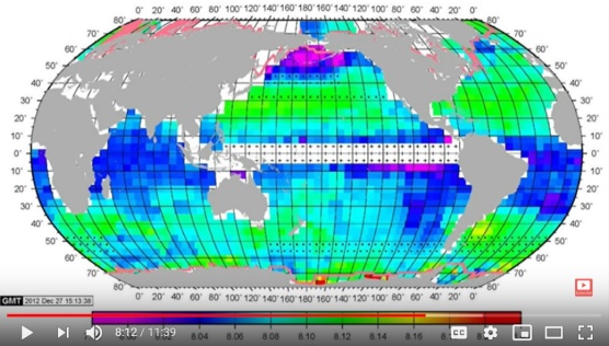
10. And what we really don’t know is how much more CO2 humans will spew our in the course of the next 50 years or so. But if we stay on the path the scientists call RCP8.5, which is the worst case representation concentration pathway, otherwise known as the business as usual scenario, which is the curve we are following at the moment, then according to the IPCC, we can expect the further lowering of the average pH by about o,3 to 0.4 by the year 2100. That will drop the pH level to about pH=7.8 which is very likely to have a negative impact on the eco system of our ocean. Here’s a pteropod swimming around in pH of 8.1 Pteropods are tiny little marine snails which are really a kind of plankton. They play a very big role in the oceanic food chain and eco system. Here is what happens when it’s put in water at pH=7.8 which is what we might get to in 2100 if we continue on the way we are. It may take a month and a half for this to happen but essentially the shell dissolves as carbonate reacts with the free hydrogen ion to make bicarbonate.
11. While we are on the RCP 8.5 business as usual, renewable energy technology is advancing at breathtaking speed and social and political will is changing fast despite the noise coming out of the White House. So it’s unlikely that we will stay on that trajectory all the way to 2100 and in fact we probably wouldn’t get there if we did. That’s not an oxymoron. A study by the Royal Society in 2014 which carried out a combined survey of the water and the pteropods along the Washington, Oregon, California coast in August 2011 shows that large portions of the shelf waters are already corrosive to pteropods. They found that 53% of the onshore and 24% of the offshore pteropods had severe dissolution damage. The study estimated that the incidence of pteropod severe shell dissolution due to anthropogenic ocean acidification has doubled in near shore habitats since pre-industrial times across this region and is on track to triple by 2050. {Bednaršek, N., et al. “Limacina helicina shell dissolution as an indicator of declining habitat suitability owing to ocean acidification in the California Current Ecosystem.” Proceedings of the Royal Society B: Biological Sciences 281.1785 (2014): 20140123, ABSTRACT: Few studies to date have demonstrated widespread biological impacts of ocean acidification (OA) under conditions currently found in the natural environment. From a combined survey of physical and chemical water properties and biological sampling along the Washington–Oregon–California coast in August 2011, we show that large portions of the shelf waters are corrosive to pteropods in the natural environment. We show a strong positive correlation between the proportion of pteropod individuals with severe shell dissolution damage and the percentage of undersaturated water in the top 100 m with respect to aragonite. We found 53% of onshore individuals and 24% of offshore individuals on average to have severe dissolution damage. Relative to pre-industrial CO2 concentrations, the extent of undersaturated waters in the top 100 m of the water column has increased over sixfold along the California Current Ecosystem (CCE). We estimate that the incidence of severe pteropod shell dissolution owing to anthropogenic OA has doubled in near shore habitats since pre-industrial conditions across this region and is on track to triple by 2050. These results demonstrate that habitat suitability for pteropods in the coastal CCE is declining. The observed impacts represent a baseline for future observations towards understanding broader scale OA effects}.
12. So what’s to make of all this complicated information? Well, ocean acidification doesn’t mean that our oceans are all full of acid so I can park my irrational fear of going swimming and melting my face but the science is telling us that the direction of travel is toward a less alkaline composition. And when a reaction like that takes place in a body of water as vast and as fundamental to life as our ocean systems then it must surely be something that we need to keep a very close eye on.

PART-2: CRITICAL COMMENTARY 

1. If ocean acidification is driven by fossil fuel emissions there ought to be a detectable statistically significant detrended correlation between emissions and oceanic CO2 concentration to establish the responsiveness of the rate of increase in oceanic CO2 concentration to the rate of fossil fuel emissions at an annual time scale. That is, years with very high rates of fossil fuel emissions should show larger increases in oceanic CO2 than years with low fossil fuel emissions. This test is carried out in a related post [LINK] . No such correlation is found in the data [LINK] . The relevant chart from the linked post is reproduced below. 
2. An additional consideration is the mass balance. In a related post oceanic CO2 concentration data 1958-2014 are presented that show average annual increase 0.002 millimoles of CO2 per liter of ocean water in the top 5000 feet of the ocean for a total increase of 0.114 millimoles/liter (MMPL) in the study period 1958-2014.
3. The total cumulative fossil fuel emissions in this period 1958-2014 was 328 gigatons. Even in the impossible scenario that all of the fossil fuel emissions ended up in the ocean uniformly distributed throughout the ocean, it could cause an increase in CO2 concentration by 0.021 MMPL. However, since the oceanic CO2 data presented above are taken from the top 5000 feet of the ocean (approximately 80% of the ocean in terms of volume), we assume that fossil fuel emissions change CO2 concentration in only the top 5000 feet of the ocean. In that case, the maximum possible increase in oceanic CO2 concentration is 0.021/0.8 = 0.026 MMPL.
4. The mass balance presented in paragraphs 2&3 above show that fossil fuel emissions cannot explain the observed change in oceanic CO2 concentration. Therefore causes other than fossil fuel emissions must be considered particularly since the the assumption in paragraphs 2&3 above that ALL fossil fuel emissions end up in the ocean is unlikely given the IPCC figures that show that CO2 in emissions go mostly to photosynthesis and increase in atmospheric CO2 concentration.
5. In addition to the the mass balance and correlation problems in the attribution of ocean acidification to fossil fuel emissions there is a vertical concentration gradient issue. If the atmosphere were the source of the CO2 found in the ocean we would expect a vertical concentration gradient with high concentration near the surface and lower concentration in deeper waters; but that is not the case. As the chart below shows, the vertical gradient shows higher concentrations in deeper waters.
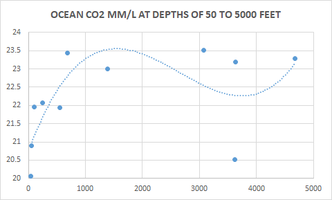
6. The analysis and evaluation of oceanic CO2 data in terms of fossil fuel emissions and atmospheric CO2 concentration is yet another extreme example of the atmosphere bias in climate science and the corruption of scientific principles with anti fossil fuel activism [LINK] . This approach to understanding the ocean ignores significant paleo data that demonstrate the impact of the ocean itself and its geological sources of carbon and heat in climate phenomena [LINK] [LINK] [LINK] [LINK] [LINK] . It is likely that the ocean acidification fear of AGW climate change is derived from the PETM event when the ocean had poisoned itself with CO2 with a horrific oxidation event involving geological carbon that depleted the oceans oxygen and caused mass extinctions that on the plus side gave rise to land based mammals from which we humans are derived. The climate science assumption that mass extinctions are a bad thing and should not be allowed to happen ignores the important evolutionary function of mass extinctions of species that are normally followed by mass explosions of new species.
7. An additional argument often made in the ocean acidification scenario is the CO2 warming feedback horror that when the acid gets to the ocean floor where dead shellfish have sequestered carbon, the acid will melt the shells and release the carbon back into the ocean-atmosphere climate system. This scenario is not consistent with the known properties of the ocean floor much of which is made of large igneous provinces that consist of basalt, a high pH basic substance that will surely neutralize the relatively insignificant amount of acid that humans can produce.
8. To summarize: No matter what kind of horror can be painted in terms of ocean acidification chemistry, until it can be shown that it is a creation of fossil fuel emissions and that it can be moderated by taking climate action in the form of changing the global energy infrastructure away from fossil fuels, the presentation has no relevance to the climate change issue. 

[LINK TO THE HOME PAGE OF THIS SITE]

[LIST OF TBGY POSTS]

THIS POST IS A CRITICAL REVIEW OF A YOUTUBE  LECTURE ON AN ICE FREE ARCTIC BY TBGY [LINK]

THIS POST IS PRESENTED IN TWO PARTS

THE FIRST PART (23 PARAGRAPHS), LABELED “TRANSCRIPT” IS A  TRANSCRIPT OF THE TBGY LECTURE

THE SECOND PART, LABELED “CRITICAL COMMENTARY” FOLLOWS THE TRANSCRIPT AND PRESENTS A CRITICAL EVALUATION OF THE TBGY PRESENTATION

FIRST PART: TRANSCRIPT OF THE LECTURE

1. At the risk of using unfortunate phraseology, Arctic sea ice has been a hot topic for many years now. The Arctic is often called the world’s air conditioning system because of the pivotal role it plays in controlling the planet’s climate largely due to the enormous ice sheet sitting on top of Greenland and the vast body of sea ice that ebbs and flows in the Arctic Ocean. So if those two bodies of ice start to diminish, then you can expect the air conditioning effect to change as well.
2. There seems to be a constant debate about accuracy of measurement up in the Arctic. The implications of single year anomalies in the dataset get disputed as does the accuracy and calibration of different measuring instrumentation, margins of error in climate modeling, and value differences from calculating techniques from one monitoring agency to another.
3. But really speaking, it doesn’t matter which organization you prefer or which dataset you choose to use from one year to another or even which graph or chart you find easiest to read. My personal favorite is Jim Pettit’s spiral graph, by the way. The trend line of every single reputable Arctic sea ice dataset, graph, and chart is an inexorable trajectory downwards toward zero.
4. And when I say zero, I should probably clarify a couple of important caveats. The first is that “zero” in climate science terms means a sea ice extent that is less than one million square kilometers. The second is that there is no suggestion that this will be a year-round phenomenon – at least in the short term anyway. It is likely that the first time we get an Arctic sea ice extent that is less than one million square kilometers it will stay that way for a couple of weeks towards the end of September before building back up again when the colder months start to encroach but the heat that will have got into the water while the ice was missing will make it extremely likely that once we’ve had a Blue Ocean Event , we’ll continue to get them every year thereafter.
5. And there is an understandable human curiosity that drives the climate science community to try to make predictions about when that zero mark might actually be reached. At one extreme end of this prediction scale 2017 was touted by some as an almost guaranteed date for the first Blue Ocean Event right up until the 2017 minimum actually arrived and the sea ice bottomed out at about 4.7 million square kilometers. At the more conservative end of the scale, organizations like our own UK Met Office point to the slowdown in the Atlantic Overturning Meridional “Currents” as an indicator of a much longer timeline perhaps to the end of the century.
6. Conversely, the American Geophysical Union or the AGU has just released a new report pointing to a long term warming phase in the tropical Pacific which they suggest may mean a Blue Ocean Event could occur in the next twenty years or so.
7. Others use different extrapolations to of graph trends to hit various possibilities. This graph of prior ice measurements from 1980 to the present day has no fewer than five different overlay fit-lines including a straight linear trend line, an exponential fit, a second order polynomial fit, a log fit, and even something called a Gompertz fit. Pick your favorite line on this graph and you can have a Blue Ocean Event anywhere from about 2024 to 2050. All of that is fascinating stuff. It’s a bit frustrating and confusing for the non-scientific on-looker.
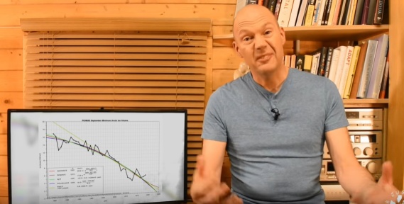
8. But attempting to put our finger on when in the next 80 years this Blue Ocean Event is likely to descend upon us is perhaps distracting us all from the real question which is what will happen after a  Blue Ocean Event and what can we do now to mitigate its worst effects. So this video contains no predictions from an English layman about Blue Ocean Event timelines. Instead we will have a look at the inextricably interconnected nature of the Arctic and its local environment and the wider global climate to establish the top ten most significant potential outcomes of an ice free Arctic.
9. The top ten most significant potential outcomes (SPO) of an ice free Arctic: SPO#1: LATENT HEAT: As long as there is ice in a body of water, then any surrounding heat energy is carried towards the ice to try and make it melt. But the energy needed to make it change state or phase from solid ice to liquid water is the same amount of energy that would heat an equivalent volume of liquid water all the way up to 79C. So that’s your first problem. Once all the ice is gone, the water gets much warmer very quickly indeed. And then you’ve got consequence #2 which is Albedo change. 
10. The top ten most significant potential outcomes (SPO) of an ice free Arctic: SPO#2: ALBEDO CHANGE: Once all the ice goes you no longer have a nice big sheet of reflective white stuff to bounce the sun’s heat safely back out into space. Back in program 17 we did a little experiment with a digital thermometer, a couple of halogen lights, and some black and white cards and it was pretty obvious that the dark cards was immediately absorbing loads more heat than the white card. And that’s exactly what happens when ice disappears from the top of a dark blue ocean. So all that energy that was previously being reflected back by the ice were now being absorbed by the water.
11. The top ten most significant potential outcomes (SPO) of an ice free Arctic: SPO#3: ALBEDO CHANGE:  ACCELERATED MELT OF THE GREENLAND ICE SHEET:  But hold on I hear you say. The Greenland Ice Sheet is on land not in the sea, so it’s a completely different thing, right? Well, yes. But the rapid warming of a continent size of water right next to the land mass means that ambient air in the region will also be getting warmed up. That warmer air will be pulled inland and across the surface of Greenland and it is this that will contribute to the accelerated melting of the ice sheet. 
12. The top ten most significant potential outcomes (SPO) of an ice free Arctic: SPO#4: ALBEDO CHANGE:  INCREASE IN WATER VAPOR:  So we’ve got more liquid water from the melting ice and we’ve got a warmer atmosphere because of the various feedback loops that we just looked at. Physics tells us that for every 1C of warming, our atmosphere can hold about 7% more moisture. So now we’ve got more water vapor in the skies directly above the Arctic and water vapor is itself a very potent greenhouse gas. As dense low clouds drape a warming blanket over the land and sea, we get ourselves one more feedback loop to add to the list. 
13. But because our global climate system is so interconnected, all the extra moisture in the air coupled with the warmer atmosphere also means a huge increase in energy to whip up storms, hurricanes, cyclones, and extreme flooding all over the world. We’ve already got just over a degree of warming compared to 1850 levels and that’s quite clearly having a big impact on extreme weather events around the world. According to a recent report from the World Meteorological Organization (WMO), most of the natural hazards that affected nearly 62 million people in 2018 were associated with extreme weather and climate events with 35 million hit by floods. Hurricane Florence and Hurricane Michael were just two of 14 $1 billion disasters in 2018 in the United States. Super Typhoon Mangkhut affected 3.4 million people and killed 134 mainly in the Philippines. Kerala in India suffered the heaviest rainfall and worst flooding in nearly a century. 
14. And all of that is without a Blue Ocean Event . The regularity and severity of these things will most likely see a very rapid increase as a result of an Ice Free Arctic and all that extra water will also result in consequence #5.
15. The top ten most significant potential outcomes (SPO) of an ice free Arctic: SPO#5: SEA LEVEL RISE : As water gets warmer, it expands and as the Greenland Ice Sheet melts at an ever increasing rate, that melting ice will flow down into the sea, an both of those things together will result in rising sea levels; not just in the Arctic but all around the globe. They are already rising as a consequence of human induced climate change of course but after a Blue Ocean Event, we’ll stop talking in tenths of millimeters a year and start talking in tens of centimeters a decade or so. And then it won’t just be hundreds of millions of people in vulnerable places like Bangladesh who suffered the loss of their homes and livelihoods as well as famines, disease, and premature deaths, something we’ve become a bit numb to here in the West because it only happens on the telly as far as we’re concerned. No, no! Now the water will coming after us comfortable affluent <people> as well. Most of the major cities in the financial centers of the world are in coastal areas and most of them face significant or even catastrophic destruction as water levels encroach on the lower lying districts. But there are some political leaders out there who wave a bit bravado about and tell their citizens they will simply use human ingenuity and technology to keep the water out. Miami for example, is already spending $500 million to install a massive pumping system to pump water back out into the ocean. And you know, good luck with that!
16. The top ten most significant potential outcomes (SPO) of an ice free Arctic: SPO#6: SEVERE JET STREAM DISRUPTION : A Blue Ocean Event will significantly accelerate the phenomenon known as Arctic Amplification for all the reasons we just talked about. The Arctic has already warmed by nearly 2C just over the last 30 years – much faster than the rest of the planet. And that is reducing the differential in temperature between the high latitudes and the equatorial region. And that causes the jet stream to slow down and meander about much more. A slower more meandering jet stream drags colder Arctic air down to lower latitudes for prolonged periods of time giving us things like The Beast from the East that we got in Europe in the year 2018; and many of the severe cold snaps that North America has been suffering in the last couple of years. But crucially, it dragged warm equatorial air much farther north way up into the Arctic Circle also for prolonged periods. So we witnessed ridiculously high temperatures like +11C in the North Pole in September. And of course that amplifies the Arctic warming still further and strengthens all the effects we’ve already looked at. 
17. The top ten most significant potential outcomes (SPO) of an ice free Arctic: SPO#7: METHANE : We’ve all probably seen headlines like the 50 Gigaton Methane Bomb; or The Ticking Time Bomb of Methane . So what’s this all about? Where is all this methane coming from? And why does it need to be included in this Blue Ocean Event consequences? The 50 Gigaton number was first brought to light by scientists specializing in the East Siberian Arctic Shelf (ESAS) as far back as 2008 during the European Geophysical Conference. The ESAS continental shelf is extremely shallow, only about 50 meters deep. In a 2013 paper by Gail Whiteman, Chris Hope, and Peter Wadhams. They explain that as the amount of Arctic sea ice declines at an unprecedented rate, the thawing of offshore permafrost releases methane. A 50 gigaton reservoir of methane stored in the form of hydrates exists on the Siberian Arctic shelf. It is likely to be emitted as the sea bed warms steadily over 50 years or so. Or suddenly! According to Peter Wadhams, even if only 8% of the methane were released, this would very rapidly add about 0.6C to our global temperature; and rapidly rising temperatures will have a DEVASTATING effect on the main food growing regions of the world.
18. The top ten most significant potential outcomes (SPO) of an ice free Arctic: SPO#8: Global Food Crisis:  Abrupt global warming will mean that “these vital food growing regions”  {Brazil, Argentina, Indian Subcontinent, China, SE Asia}, will begin to experience such extreme temperatures and weather that agriculture will become practically impossible. The report in Time Magazine [LINK]  summarizes the predicament very well. Globally we rely on a very slender thread of genetic diversity. More than 50% of all human calories come from just three plants – rice, maize, and wheat. And the rice maize and wheat come from {Brazil, Argentina, Indian Subcontinent, China, SE Asia} all of these regions are going to be MASSIVELY affected by climate change and global warming – especially following the Blue Ocean Event. Our current human activity puts us on a path toward 4C warming above pre-industrial by the year 2100.  The map of the world at that stage will look something like this.
19. It is noted in the map above that Canada will grow most of the world’s crops, Northern Europe under huge pressure for habitable land, Russia has arable land and a habitable zone, the SW USA is a desert, North Africa, the Middle East, and Southern USA are uninhabitable, Africa is mostly desert, Southern Europe suffers from desert encroachment, Southern China is an uninhabitable dust bowl, Amazonas is an uninhabitable desert, Bangladesh and South India are abandoned after Himalayan glaciers have melted, Australia is useful only for Uranium mining, and Patagonia remains an arable zone.
20. So the comfortable insulation and detachment we currently enjoy in the West will be pretty much shattered as we struggle to find enough food to feed our population. Here in the UK for example, we get 50% of our food from outside the country much of which is sourced from these vulnerable countries. And these huge swaths of once fertile land now turns into a dust bowl with summer temperatures exceeding 50C, a temperature way to high to grow anything. They will become places where human activity is more or less impossible.
21. The top ten most significant potential outcomes (SPO) of an ice free Arctic: SPO#9: CLIMATE REFUGEE CRISIS:  Commentary from Alfredsdottir, Icelandic lawmaker and former Minister of Foreign Affairs in a 2017 NATO report. It says that the refugee crisis shaking political stability throughout much of the Middle East and posing serious problems in Europe could be a harbinger of things to come. The huge economic and social costs linked to mass movements on this scale are self evident. It is distinctly possible that global climate challenges could trigger mass movements particularly in regions which no longer have the water and agricultural resources needed to support life. 
22. The top ten most significant potential outcomes (SPO) of an ice free Arctic: SPO#10: REGIONAL AND GLOBAL CONFLICT.  In that same NATO report, Philippe Vitel, French legislator, says that it is a moral imperative to reduce hunger and thirst in the world. But it is also a strategic imperative. If the Middle East and North Africa cannot achieve sustainable food and water security, we will see many more crises in the years to come. Alfredsdottir concludes that the potential for conflict between regions affected by climate change should not be ruled out. And that’s ultraconservative NATO speaking, not Greenpeace or Friends of the Earth. 
23. Of course none of these consequences represents an existential threat to the planet itself . Our earth doesn’t care what the temperature is or what the relative concentration of the greenhouse gases in the atmosphere are. Its self regulatory systems have always re-calibrated themselves over long periods of time so that they always get back to equilibrium. The point is that for the last 11,000 years, since the dawn of human civilization, we’ve been able to design our entire societal infrastructure in every corner of the globe about a remarkable stable and predictable climate with an average global temperature that has never varied by more than 0.4C in all of that time until now. Our governments are perfectly well aware of what lies ahead but they are not taking the radical actions necessary partly in fear of the fossil fuel money that controls the modern political landscape, and partly in fear of inducing panic and unrest amongst their population. So thet need to be shown that their populations do want them to take radical action. That’s the objective of groups like 350.org and Extinction Rebellion.  And not forgetting of course the kids school strike movement inspired by the astonishingly determined and focused Swedish teenage activist Greta Thunberg. You might feel there is very little you can do as an individual to mitigate such an enormous issue but that doesn’t mean there is nothing you can do at all. If you feel it’s within your gift, get involved with one of these groups or the very least hassle your elected representative and don’t take no for an answer. On a practical level, take your money away from those doing harm. Change your energy supply to a green energy supplier or better still get solar powers on your roof. And don’t give up if you live in an apartment block. Get together with the other residents and sort out a communal system. That’s already happening in many European cities. Change your bank, your life insurance, your pension provider if you’ve got one, to an organization that has divested all its funds away from fossil fuels. If you can, get rid of your internal combustion engine car and walk or cycle wherever possible. And if you do need to have a car from ability reasons or you’ve got 5 kids, then the next time you buy a new one, make sure it’s an electric vehicle. Change your diet to minimize the amount of meat you consume specially beef. A kilogram of beef is 30x more impactful on the environment than a kilogram of plant protein. Ideally, move to a plant based diet altogether. It’s much cheaper and it’s far healthier for you anyway. Each of us has a personal choice to make about how we respond to this climate crisis. I know a lot of you out there are really taking positive actions of your own.

SECOND PART: CRITICAL COMMENTARY

HYPOTHETICAL NATURE OF THE BLUE OCEAN EVENT:

In paragraph #3 above, TBGY says that the long term trend of year to year changes in September minimum sea ice extent is “an inexorable trajectory downwards toward zero” with the clarification that anything under 1E6 sq-km of Arctic sea ice extent counts as zero and that this state of Arctic sea ice extent, previously called the ICE FREE ARCTIC is described by TBGY as a Blue Ocean Event (BOE). After quoting some forecasts about when the BOE might happen, TBGY admits that all prior forecasts of the BOE have turned out to be wrong.

The long list of failed BOE forecasts is presented in a related post as “the ice free Arctic obsession of climate science” [LINK] and a recent forecast of the BOE {Thackeray, Chad W., and Alex Hall. “An emergent constraint on future Arctic sea-ice albedo feedback.” Nature Climate Change 2019} is discussed. Like TBGY, the paper acknowledges failures of prior BOE forecasts but attributes these failures to deficiencies in climate models that the authors claim have now been corrected by re-calibrating climate models with the deep seasonal cycle of sea ice extent. Based on the re-calibration, the authors predict an ice free Arctic (BOE) at some time between 2044 and 2067. Unlike prior forecasts of an ice free Arctic (BOE), this forecast uses a long time horizon of more than 20 years into the future and a large error margin > 20 years. It is a sign that climate science is now weary and apprehensive of the BOE game having failed so many times in the past.

In this lecture, TBGY takes a very different and radical approach in the strategy to continue the BOE game in the face of dramatic and humiliating failures of the past and it is in this context that he says in paragraph#5 above that “And there is an understandable human curiosity that drives the climate science community to try to make predictions about when that zero mark might actually be reached. At one extreme end of this prediction scale 2017 was touted by some as an almost guaranteed date for the first Blue Ocean Event right up until the 2017 minimum actually arrived and the sea ice bottomed out at about 4.7 million square kilometers. And now the AGU forecasts the BOE in 20 years and the UK Met Office projects a BOE by end of the century. These statements are an acknowledgement of the failure of climate science to predict the BOE.

It is here and in this context, that TBGY makes the defining statement of this lecture when he says that {attempting to put our finger on when in the next 80 years this Blue Ocean Event is likely to happen is distracting us all from the real question which is what will happen after a  Blue Ocean Event and what can we do now to mitigate its worst effects. So this video contains no predictions about Blue Ocean Event timelines. Instead we will have a look at the inextricably interconnected nature of the Arctic and its local environment and the wider global climate to establish the top ten most significant potential outcomes of an ice free Arctic}. THEREFORE THIS LECTURE DESCRIBES A HYPOTHETICAL STATE OF THE WORLD AFTER A BOE HAS OCCURRED. THIS HYPOTHETICAL STATE OF THE WORLD IS DESCRIBED IN TERMS OF The top ten most significant potential outcomes (SPO) of an ice free Arctic. TBGY identifies the top ten climate consequences of a BOE as: SPO#1: LATENT HEAT: SPO#2: ALBEDO CHANGE: SPO#3: ACCELERATED MELT OF THE GREENLAND ICE SHEET:  SPO#4: INCREASE IN WATER VAPOR: SPO#5: SEA LEVEL RISE:  SPO#6: JET STREAM DISRUPTION : SPO#7: METHANE: SPO#8: Global Food Crisis: SPO#9: CLIMATE REFUGEE CRISIS: SPO#10: REGIONAL AND GLOBAL CONFLICT, as described above.

Though the ten “consequences” of a hypothetical Blue Ocean Event are painted in horrific terms in over-hyped fear mongering language, the reality is that none of these events have happened and none is likely to happen because they are projections of a purely hypothetical scenario. What the actual data show is a repetitive pattern of failed high pitched alarms about an imminent and catastrophic ice free Arctic in September. This pattern can be traced from at least as far back as 1999. An unacceptable number of these alarms have been invoked on a regular  basis since then and all of them, except for the ones that are still in the future, have been proven false [LINK] .

The BOE alarm about an ice free Arctic in September assumes that the observed year to year decline in September Minimum Sea Ice Extent (SMSIE) in the Arctic is driven by fossil fueled AGW and that therefore it can and must be attenuated by reducing or eliminating the use of fossil fuels. Yet, the required relationship between climate change warming and SMSIE has simply been assumed. No supporting empirical evidence has been provided. In fact, no such evidence exists. As shown in related posts on this site, correlation analysis between surface temperature and SMSIE does not show that that SMSIE is responsive to changes in AGW surface temperature [LINK]  [LINK] . The single-minded obsession of climate science with fossil fuel emissions [LINK] makes it impossible for the science to include natural geological sources of heat in their analysis of ice melt phenomena even in regions known to be geologically active [LINK] [LINK] [LINK] . 

CONCLUSION

That climate science must now resort to a hypothetical BOE scenario to present the fear of AGW in terms of the alarming “consequences” of the BOE is not evidence of things to fear but an admission of the failure of the science. The science is proven wrong and its forecasts of the horrors of an ice free Arctic are discredited.

The admission of these failures and the attempt to sell the fear of hypothetical future horrors of climate change in the face of such failure is yet another example of an assumption in climate science that the less they know the greater the fear of the potential cataclysmic impacts of climate change [LINK] . 

This logic derives from the oddity that catastrophic AGW climate change and the urgent need for climate action constitute the null hypothesis in climate science; with the alternate hypothesis being the negation of this scenario. If climate science really were a science the hypotheses would have been in reverse.

It is this trickery of climate science and the consequent use of the “shift the burden of proof ” fallacy that appears to preserve the scientific credentials of a failed science. The continued survival of such a failed science is aided by the popular press with fear based activism and a faux argument that consensus proves the correctness of the climate science theory of catastrophic AGW climate change and the urgent need to move the world’s energy infrastructure away from fossil fuels [LINK] . 

PRINCIPLES AND PRECEPTS OF ECO FEAROLOGY

PRINCIPLE #1: THE NATURAL AND THEREFORE THE DESIRABLE STATE OF THE PLANET  IS ONE WITH NO HUMANS ON IT:

A clean and pure pristine primeval planet earth existed for a billion years in natural perfection, wholeness, and wholesomeness – unpolluted, untainted, untarnished and uncorrupted in the perfection of the harmony of nature. 

1. The geology, biology, and climatology were in a state of perfection.
2. The climate was stable and unchanging with no extreme weather.
3. Living creatures both plants and animals lived in peace and tranquility as essential elements of nature itself.
4. There was no ozone depletion, no climate change, no skin cancer, no hurricanes and no species extinction from bad weather.
5. Modern day ecofearology is a yearning of humans for this humanless state of nature – a yearning by humans for a return to what the planet was like before humans came along.

PRINCIPLE #2: HUMANS ARE POLLUTION:

Meanwhile a planet far far away was being poisoned to death by evil humans. After their planet died from fossil fuel poisoning these humans set out to find a new planet to live on. They found the planet earth.

1. The devil thus appeared on earth in the form of humans who came on spaceships from outer space . Humans are not part of nature but an external force alien to nature and an abomination. They will soon turn this heavenly planet into a living hell with human activity because their nature is to consume and destroy.
2. At first the alien humans were relatively harmless living off the land as hunter gatherers in harmony with nature. But they were just biding their time and waiting for their numbers to grow.
3. When their population reached 6 million, they made their first move for the conquest of the planet. It was a fundamental change in human behavior that has come to be called the Neolithic Revolution.
4. In the Neolithic Revolution, the humans gave up their eco-friendly hunter-gatherer lifestyle and cleared forests to build homes and farms and to grow crops and raise animals in an extensive and intensive land use change that would forever alter the ecology of the earth. The strategy was immensely successful for the humans who now commanded incredible wealth and power over all other life forms. Their numbers grew rapidly in a population explosion from 6 to 60 million.
5. By the year 1750 the population of humans had surged to one billion. Their affluence from agriculture, tool-making, medical care, and new knowledge about the earth had rapidly increased their power against nature. But the greater and more devastating change was yet to come in the form of the Industrial Revolution.

PRINCIPLE NUMBER 3: THE INDUSTRIAL REVOLUTION OF THE HUMANS IS THEIR GREATEST ECOLOGICAL EVIL: 

The Industrial Revolution was made possible by the humans with a transition in their source of energy from animal power, wind, and running water to machines burning hydrocarbon fuels dug up from under the ground.

1. This new found energy source and the machines that burnt this new energy source gave the humans immense power that will create a population explosion of humans and a power the humans can use to kill the planet. Nature is now at their mercy.
2. By the year 1950, the population of humans had more than doubled to 2.5 billion and more and more machines were invented so that almost everything the humans did was driven by fossil fueled machines. These included cars and trucks for surface transportation, fossil fueled ships for crossing the oceans, and fossil fueled aircraft for their conquest of the atmosphere.
3. Nuclear bombs were invented, tested, and used. Space travel was opening up new tools and ways for humans to conquer nature. The Anthropocene was now in full force. Whereas humans had once been at the mercy of nature, the tables had been turned, and nature and the planet itself were now at the mercy of the humans and human activity.

PRINCIPLE NUMBER 4: THE PLANET IS THREATENED BY THE DISASTROUS CONSEQUENCES OF THE INDUSTRIAL REVOLUTION:

The consequences of these changes and of the implications of the complete capture of nature by humans for the ability of nature to sustain humans in the future are the primary concerns of the new science of Ecofearology. The science involves the study of nature and human activity as a way of protecting nature and managing nature to preserve its ability to sustain humans. The study of Ecofearology is guided by nine foundational PRECEPTS that provide the guidelines needed to understand the human impact on nature.

1. PRECEPT#1: There are no natural or cyclical changes on earth. All measured changes in nature are trends, all trends are human caused, and therefore all trends are bad with potentially catastrophic consequences for life on earth and the planet itself. This precept applies to the concentration of all chemicals in the atmosphere and ocean, the number of creatures of any given species, and the number of events such as storms, droughts, floods, wildfires, heat waves, cold waves, glacial retreat, and glacial advance.
2. PRECEPT#2: Regarding such trends: If it is going up it’s a bad thing and its accretion is caused by human activity. Higher levels of this thing will be the end of the world. Therefore urgent climate action is needed to save the planet. 
3. PRECEPT#3: If it is going down it’s a bad thing and its depletion is caused by human activity. Lower levels of this thing will be the end of the world. Therefore urgent climate action is needed to save the planet.
4. PRECEPT#4: All human caused trends lead to catastrophic results for the environment and by extension, the planet itself. It is not possible for a human caused trend to benefit the planet because humans are not part of nature but space aliens and unnatural.
5. PRECEPT#5: Human scientists can save the planet from the other humans because the impact of bad human intervention in nature can be undone only by the impact of good human intervention as prescribed by the human scientists because human scientists know the science and care about nature. Therefore, human intervention is necessary to save the planet from human intervention.
6. PRECEPT#6: Even if human science deniers find fault with the science of human caused catastrophe, we must ignore the human science deniers because we can’t take the chance that the human scientists could turn out to be right.
7. PRECEPT#7: If you don’t find any human caused planetary emergency that threatens the destruction of Nature and the world, it is because you have not looked closely enough. You must work harder and keep looking until you find it.
8. PRECEPT#8: The human invaders of this once pristine planet are now the managers of nature and the operators of the planet. Therefore we humans must take care of nature and run the planet because nature can no longer take care of itself like it once did now that the human invaders are here.
9. 

IT IS HOPED THAT ONCE ALL HUMANS LEARN AND UNDERSTAND THESE PRINCIPLES AND PRECEPTS OF ECO FEAROLOGY, THEY WILL FULLY SUPPORT HUMAN CLIMATE SCIENTISTS AND HELP THEM TO SAVE THE PLANET FROM US NON-SCIENTIST HUMANS. 

THANK YOU FOR HELPING AND HAVE A GOOD NIGHT.