ECS: Equilibrium Climate Sensitivity

Posted by: chaamjamal on: May 6, 2018

• In: Uncategorized
• 26 Comments

 

FIGURE 1: LARGE RANGE OF SENSITIVITY ESTIMATES IN THE LITERATURE

 

FIGURE 2: STABILITY OF ECS: MOVING 60-YEAR WINDOW

 

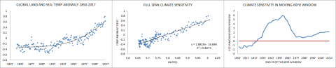
FIGURE 3: STABILITY OF ECS: SPLIT HALF TEST

 

FIGURE 4: STABLE REGRESSION COEFFICIENT AT HIGH CORRELATION

 

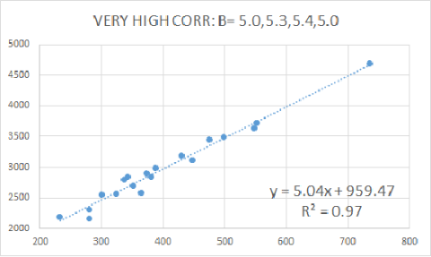
FIGURE 5: UNSTABLE REGRESSION COEFFICIENT AT LOW CORRELATION

 

RELATED POST: THE GREENHOUSE EFFECT OF ATMOSPHERIC CO2

RELATED POST: SPURIOUS CORRELATIONS IN CLIMATE SCIENCE

RELATED POST: TRANSIENT CLIMATE RESPONSE

 

1. Climate sensitivity described by Jule Charney as the expected temperature increase for a doubling of atmospheric carbon dioxide assumes that surface temperature is responsive to atmospheric CO2 concentration in accordance with the so called “greenhouse effect”. Such responsiveness implies a linear relationship between surface temperature and the logarithm of atmospheric carbon dioxide concentration. In the observational data, this responsiveness can be measured as the linear OLS regression coefficient of surface temperature to log(CO2) and then converted to the Charney doubling convention with the appropriate ratio. For example, if natural logarithm is used, the regression coefficient must be multiplied by ln(2)=0.693147 for the conversion to the Charney format.
2. In theory the Charney climate sensitivity, also called the Equilibrium Climate Sensitivity or ECS, is a universal constant. In the ideal scientific process, climate models would use the radiative forcing computations to predict the theoretical value of ECS (as Charney has done) and the testable implication of theory, that surface temperature is responsive to the logarithm of atmospheric CO2 concentration in the observational data at an annual time scale, should yield a value that is in agreement with the theoretical prediction of the climate model. This procedure has not worked out very well for the ECS because of a wide range of ECS values both for theoretical predictions by climate models and for empirical tests with the observational data of global warming.
3. In 1979, Jule Charney used the Manabe climate model, now considered dated and no longer used, to predict a symmetrical Gaussian distribution of ECS defined by a mean of ECS=3 and a 90% confidence interval of 1.5<ECS<4.5. This range was adopted by the IPCC and has since become gospel in both the literature and in textbooks. Charney died shortly after his landmark climate sensitivity presentation of 1979 but his estimate of ECS=[1.5,4.5] survives to this day as the IPCC standard against which all estimates must be compared. These comparisons have frustrated climate scientists because of a large range of values observed in climate models, in the observational data, and in climate models constrained by data both paleo and observed.
4. Figure 1 shows that ECS estimates since Charney indicate that the distribution is not symmetrical Gaussian but skewed right and also that the range of observed values is much greater than that implied by the Charney/IPCC 90%CI of ECS==[1.5,4.5]. Values of ECS=0 to ECS=10 are seen in the full range of Figure 1. The studies listed in Figure 1 are described in a related post: greenhouse effect. 
5. Figures 2&3 are taken from an empirical study of ECS using the HADCRUT4 temperature anomaly reconstructions from the instrumental record 1850 to 2017 in conjunction with Mauna Loa atmospheric CO2 measurements 1958-2017 and Law Dome CO2 estimates 1850-1957. The full text of the study may be downloaded either from SSRN.COM  or from ACADEMIA.EDU. The last frame of Figure 2 shows ECS estimates in a moving 60-year window ending in the year 1910 to 2017. The ECS value estimates in the 60-year moving window vary from ECS<0 to ECS>6, a much larger range than and inconsistent with the Charney/IPCC standard. The observed variance implies that empirical ECS estimates are unstable and a function of location within the data time series.
6. This intuition is confirmed in Figure 3 where the three columns marked BOTH are of interest in this discussion because they relate to global temperature. They display the results of a split half test for regression stability which compares ECS values for the full span, the first half of the span, and the second half of the span. The observed values are ECS=0.54 for the first half 1850-1933, and ECS=2.71 for the second half 1934-2017. From the results in Figures 2&3, taken together we may conclude that the OLS linear regression coefficient for temperature against atmospheric CO2 concentration is unstable. Such instability implies an insufficient correlation exists at the time scale of interest for the further interpretation of the coefficient in terms of its information content. In other words, the regression coefficient does not contain useful information because an insufficient correlation exists between surface temperature and log(atmospheric CO2) at an annual time scale.
7. Figures 4&5 demonstrate the stability issue. In Figure 4 there is a high correlation between X&Y at an annual time scale. There we find that random sub-spans in the time series generate regression coefficients very close to each other. The observed values in four different sub-spans are 5.0, 5.3, 5.4, and 5.0. In the low correlation case shown in Figure 5, the four random sub-span regression coefficients are very different not unlike the ECS uncertainty issue demonstrated in Figures 1,2,&3. When the correlation is low five random sub-spans yield regression coefficients of 2.4, 7.1, 1.8, 5.3, and 4.1. These two figures demonstrate that without correlation, the regression coefficient is unstable across the span of the time series whereas when the variables are correlated a stable coefficient is seen. The instability of the correlation coefficient is an indication that it is specious and that therefore it has no interpretation in terms of the phenomenon being investigated in terms of the regression coefficient.
8. In a related study, the satellite temperature measurement era 1979-2017 are used in conjunction with Mauna Loa CO2 data. These data sources are considered to be the most reliable. The results show that the correlation in the observational data between surface temperature and the logarithm of atmospheric CO2 is spurious and an artifact of shared long term trends.  When detrended, no evidence is found that surface temperature is responsive to atmospheric CO2 concentration at an annual time scale. The full text of this study may be downloaded from SSRN.COM  or from ACADEMIA.EDU. These results suggest that there is no empirical basis for the existence of an ECS climate sensitivity parameter that determines surface temperature according to atmospheric CO2 concentration.
9. The confusion and disarray in the research effort to determine the value of the ECS can thus be explained as a search for a parameter for which the assumed correlation does not exist in the data. There is some evidence of the frustration of climate science with the ECS parameter in terms of their eagerness to move away from ECS Climate Sensitivity to TCR Transient Climate Response to establish the relationship between emissions and warming. This shift is described in a related work available for download. FULL TEXT DOWNLOAD: SSRN.COM ACADEMIA.EDU
10. A parody demonstration of the failed ECS research effort is presented with data for homicides in England and Wales. It is shown that an Equilibrium Homicide Sensitivity (EHS) can be computed for the increase in homicides for a doubling of atmospheric carbon dioxide but upon further examination the correlation on which the EHS is based is shown to be specious. The full text of this study may be downloaded from SSRN.COM or ACADEMIA.EDU

 

RELATED POSTS

The Anomalies in Temperature Anomalies

The Greenhouse Effect of Atmospheric CO2

ECS: Equilibrium Climate Sensitivity

Climate Sensitivity Research: 2014-2018

TCR: Transient Climate Response

Peer Review of Climate Research: A Case Study

Spurious Correlations in Climate Science

Antarctic Sea Ice: 1979-2018

Arctic Sea Ice 1979-2018

Global Warming and Arctic Sea Ice: A Bibliography

Global Warming and Arctic Sea Ice: A Bibliography

Carbon Cycle Measurement Problems Solved with Circular Reasoning

NASA Evidence of Human Caused Climate Change

Event Attribution Science: A Case Study

Event Attribution Case Study Citations

Global Warming Trends in Daily Station Data

History of the Global Warming Scare

The dearth of scientific knowledge only adds to the alarm

Nonlinear Dynamics: Is Climate Chaotic?

The Anthropocene

Eco-Fearology in the Anthropocene

Carl Wunsch Assessment of Climate Science: 2010

Gerald Marsh, A Theory of Ice Ages

History of the Ozone Depletion Scare

Empirical Test of Ozone Depletion

Ozone Depletion Chemistry

Brewer-Dobson Circulation Bibliography

Elevated CO2 and Crop Chemistry

Little Ice Age Climatology: A Bibliography

Sorcery Killings, Witch Hunts, & Climate Action

Climate Impact of the Kuwait Oil Fires: A Bibliography

Noctilucent Clouds: A Bibliography

Climate Change Denial Research: 2001-2018

Climate Change Impacts Research

Tidal Cycles: A Bibliography